Lecture 1 - Projectile Motion

A note about kinematic equations and notation.

Be sure you check out the Pre-Course page that shows the maths and physics skills and knowledge expected at the start of this course.

In your pre-university education you will have met the kinematic equations before but most probably under another name: the suvat equations. I am not going to use the suvat notation because it is rather limiting, and instead I will introduce you to a more typical notation convention that will apply to many other fields in physics.

You will see more of why I am avoiding the suvat terminology and approach in Lecture 2. Something for you to look forward to.

The new suvat

I present to you the kinematic equations in Table 1 below. Take a few moments to look at them and compare to the suvat forms you most likely have ingrained in your memory by your teachers.

Table 1 Kinematic equations for a body moving in the \(x\) direction with constant acceleration \(a\).

KE I	\(v(t)=v_0+at\)
KE II	\(x(t) = x_0 + v_0t + \dfrac{at^2}{2}\)
KE III	\(v(t)^2 = v_0^2 + 2ax(t)\)

The form of the equations should be familiar but some of the notation may be different. By using the notation of \(v(t)\) and \(x(t)\) for velocity and position at time \(t\) respectively we are recognising that these are functions and therefore can be used to calculate the velocity and/or position at any time so long as we have an initial condition. These conditions are \(v_0\) and \(x_0\) for initial velocity and position respectively - as we will see in Lecture 2 the initial conditions terminology relates to how we solve differential equations, but you will see more of these later and in your maths courses.

Parabolic Path

You may have already learned about projectile motion in your pre-university studies but typically the approach taken is to consider only the “special points” of the projectile, namely the maximum height, range and time of flight. You may have also looked at these parameters again in the situation where the landing height is different to the firing height.

Instead of taking this approach we are going to consider the entire path of the projectile. In doing this we can easily determine the expressions for the special points you have already seen but also any other point on the path. We’ll go through an example under Example: Coconut shy cannon below which should demonstrate why modelling the entire projectile path is more versatile. Also by modelling the projectile path we can also calculate the range when fired up a slope, or a curved hill, or whetever type of ramp shape you can model with a function.
Exciting, no? You’ll have to contain your enthusiam until later for that.

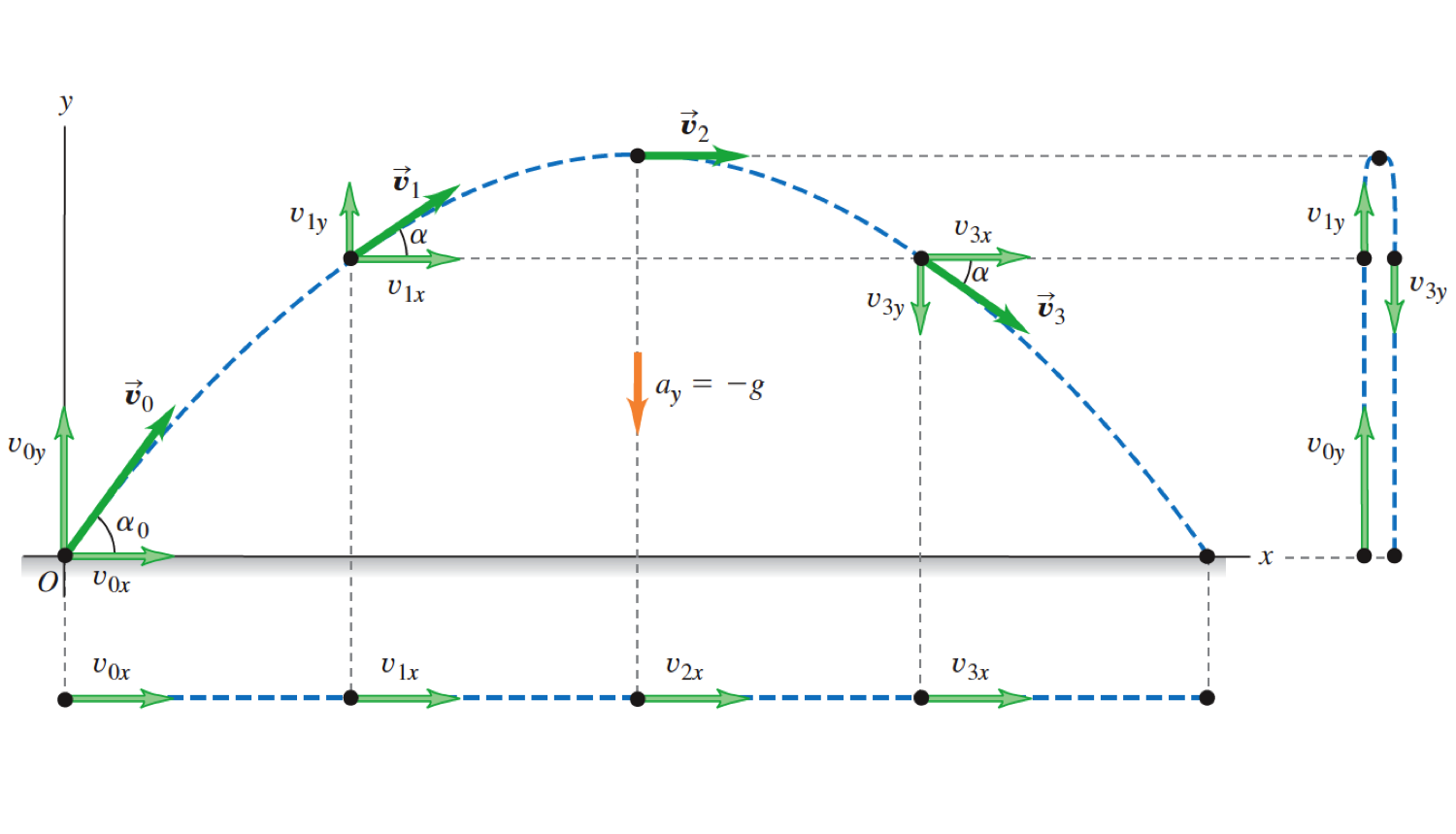
Fig. 1 A simple projectile with the same firing and landing height. The velocity vectors at the points on the path indicated are resolved into their horizontal and vertical components. Note that the only acceleration is due to gravity - air resistance is neglected.

Note

By simple I mean the firing height and landing height are the same, and we are assuming there is no air resistance.

In Fig. 1 above we can see a simple projectile path for a particle fired at some angle \(\theta\) with some initial velocity \(v_0\). It is worth noting that the textbook this image comes from (Young and Freedman) uses \(\alpha_0\) for initial firing angle with respect to the horizontal and \(\alpha\) for angles to the horizontal at any other point along the path. I find this a bit unusual and will stick to using \(\theta\) for the angles, and generally I’m just interested in \(\theta_0\). Even though the figure shows the velocities (total, \(x\) and \(y\) components) at different positions, all we need to know is \(v_0\) and \(\theta\) in order to create a model that describes the entire projectile path.

We can use the horizontal component of the firing velocity \(v_{0,x}\) and initial vertical component \(v_{0,y}\) along with some basic trigonometry to find

(2)\[\begin{equation} \cos\theta=\frac{v_{0,x}}{v_{0}}\quad \mathrm{and}\quad \sin\theta=\frac{v_{0,y}}{v_{0}} \end{equation}\]

and a little rearrangement gives

(3)\[v_{0,x}=v_{0}\cos\theta\quad\mathrm{and}\quad v_{0,y}=v_{0}\sin\theta\]

Note

KEII is \(x(t) = v_0t + \dfrac{at^2}{2}\) from Table 1

We can now use KE II (twice, once for horizontal and once for vertical) to determine the \(x\)- and \(y\)-positions of the particle as a function of time.

Horizontal: Since the only acceleration involved here is due to gravity the horizontal acceleration \(a_{x}=0\). So the horizontal part of equation (3) gives

(4)\[x=v_{0,x}t=\left(v_{0}\cos\theta\right)t\]

Vertical: Gravity is the only cause of acceleration and it acts in a downwards direction, and so \(a_{y}=-g\) (initially rising object). From equation (3) we find

(5)\[y=v_{0,y}t-\frac{1}{2}gt^{2}=\left(v_{0}\sin\theta\right)t-\frac{1}{2}gt^{2}\]

We now have two equations that define the position vector of the particle \(\textbf{r}(t)\) at any time \(t\), i.e.

(6)\[\begin{equation} \textbf{r}(t)=\left(\begin{array}{c} \left(v_{0}\cos\theta\right)t\\ \\ \left(v_{0}\sin\theta\right)t-\frac{1}{2}gt^{2} \end{array}\right) = \left(v_0\cos\theta\, t\right)\, \hat{\textbf{i}} + \left((v_{0}\sin\theta)\,t-\frac{1}{2}gt^{2}\right)\, \hat{\textbf{j}} \label{eq:Vector equation of parabola} \end{equation}\]

Although this is a nice compact way of describe the position of the particle it is limited in use, particularly for what we want to do next. What is more useful is if we rearrange equation (4) to express \(t\) in terms of \(x\) \(\left(\text{i.e. }t=\dfrac{x}{v_{0}\cos\theta}\right)\), and substitute this expression for \(t\) into equation (5) to obtain

(7)\[\begin{split}y&=\left(\frac{v_{0}\sin\theta}{v_{0}\cos\theta}\right)x-\left(\frac{g}{2v_{0}^{2}\cos^{2}\theta}\right)x^{2}\nonumber\\ &=x\tan\theta-\frac{gx^2}{2v_{0}^{2}\cos^{2}\theta}\end{split}\]

We now have an expression that allows us to find the \(y\)-coordinate of a particle in a projectile path at any given \(x\)-coordinate, and vice versa. Note that the general equation of a parabola is \(y=ax-bx^{2}\), so equation (7) follows the form we would expect for a projectile.

Example: Coconut shy cannon

This may seem more difficult than the approach you are used to in calculating the “special points”, so let us now think about a trip to the fairground where we can put our general model for a projectile to the test.

You arrive at a fairground attraction and the person on the stall explains the challenge before you. A coconut is standing on a pole, you are given a small toy mortar launcher that has a fixed firing angle and a constant firing velocity. Your challenge is to position the mortar launcher on the floor at the appropriate distance so that the projectile hits the coconut off the pole when it is fired. You win a cuddly toy if successful!

As this is a hypothetical scenario we will make some simplifications but you can build on this in the future to better approximate the real world situation. Our assumptions are

1. There is no air resistance

2. Both the projectile and the coconut are point masses

3. The height of the mortar launcher is sufficiently small that we assume it fires from ground height.

Note

Seriously. Every time you try a problem without a well labelled diagram a llama somewhere sheds a tear.

We first need to set up our simplified scenario. The best and most important starting point is to draw a well labelled diagram. We need our diagram to include information about the projectile as well as the relative position on the coconut on the pole. Fig. 2 shows how I would draw the diagram for the problem we are trying to solve.

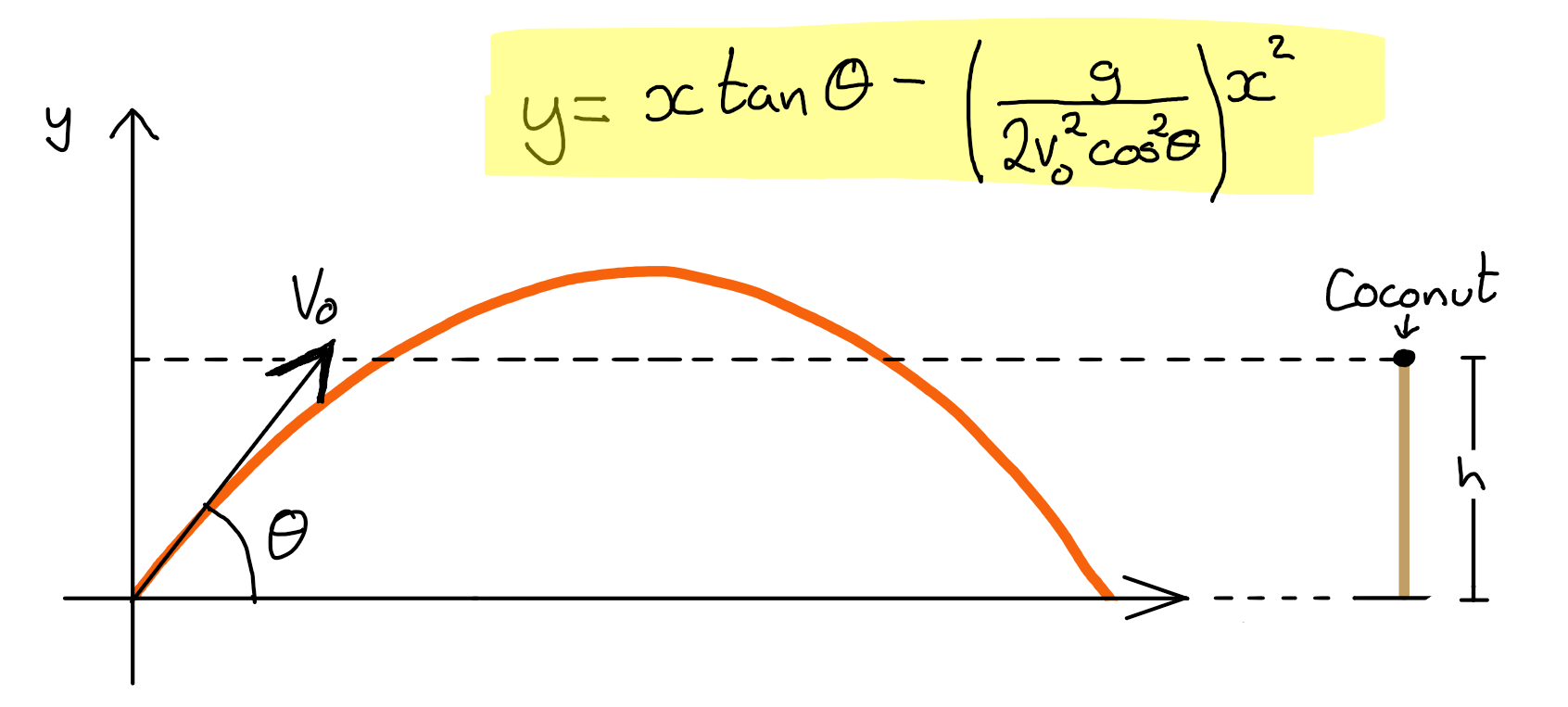
Fig. 2 A simple projectile with a coconut on a pole of height \(h\). The horizontal dashed line indicating the height of the coconut intersects the parabolic path of the projectile at two points, the \(x\) coordinates of which are the solutions found in equation (8)

There are two ways to think about the solution to this problem, although in reality they are two different ways of saying the same thing. The first is the physics / real world view where we are wanting to find when the projectile has the same height as the coconut. Alternatively we can think more mathematically and see this as the intersection of two curves, one for the parabola and the other for a straight horizontal line at \(y=h\).

So we can set \(y=h\) into equation (7) which means we can now solve to find the horizontal distance between the launch point and the coconut. Thus

\[\begin{align*} h &= x\tan\theta - \dfrac{gx^2}{2v_{0}^2\cos^2\theta}\\ 0 &= x^2 - \dfrac{2v_{0}^2\cos^2\theta\tan\theta x}{g} + \dfrac{2v_{0}^2\cos^2\theta h}{g} \end{align*}\]

which has been rearranged into the quadratic form with \(a=1\), \(b=-\dfrac{2v_{0}^2\sin\theta\cos\theta}{g}\) and \(c=\dfrac{2v_{0}^2\cos^2\theta h}{g}\).

You should all be familiar with the quadratic formula for solving a second order polynomial, and the reason I have rearranged my equation for the projectile is that having \(a=1\) makes the final equation neater. Remember the quadratic formula has \(2a\) in the denominator, so this trick of rearranging saves me having a complicated denominator and also means I can simply ignore the \(a\) terms. So finally we get

(8)\[\begin{split} x &= \frac{1}{2}\left(-b \pm \sqrt{b^2 -4c}\right)\nonumber\\ &= \frac{1}{2}\left(\frac{2v_0^2\sin\theta\cos\theta}{g}\pm\sqrt{\frac{4v_0^4\sin^2\theta\cos^2\theta}{g^2}-\frac{8v_0^2\cos^2\theta h}{g}}\right)\nonumber\\ &=\frac{1}{2}\left(\frac{v_0^2\sin(2\theta)}{g} \pm \sqrt{\frac{8v_0^2\cos^2\theta}{g}\left[\frac{v_0^2\sin^2\theta}{2g}-h\right]}\right)\end{split}\]

The plus-minus \((\pm)\) means that we have two solutions which should come as no surprise when we look back at Fig. 2. The two solutions correspond to hitting the coconut on the way up (left of the maximum point) and on the way down (right of the maximum point).

As useful as this general expression is, we need to be careful and consider the limitations. The square root component provides the main breaking point. If the expression within the square root is negative we have no (real) solution. But never fear! We can turn this around and actually make some use of this apparent limitation to tell us a bit more about the system.

If we want the expression within the square root sign to always be zero or positive then we can state the requirement that

\[\begin{align*} 0 &\leq \left(\frac{v_0^2\sin^2\theta}{2g}-h\right) \end{align*}\]

as the term outside the square brackets can never be negative. With some slight rearrangement we can impose an upper limit on \(h\) plus taking the real world lower limit of \(h=0\) because the coconut needs to be at or above ground, we find

(9)\[0 \leq h \leq \frac{v_0^2\sin^2\theta}{2g}\]

This is kind of interesting now but it will be even more so when we have a little bit more information from the next section. So let us press on.

“Special points’’

You may be wondering why you were only taught to find the three “special points”. That is a conversation about the school education system that I will not go into here but we will now see that these three points can be found from the general form of a projectile path given in equation (7).

Maximum height, \(h_\text{max}\)

From Fig. 1 it should be clear that the point of maximum height is the stationary point of the parabolic curve. Whenever you hear the phrase “stationary point” you should always think calculus which in this circumstance means remembering that a stationary point has a gradient or first derivative equal to zero. Working it through from equation (7) we find,

(10)\[\begin{align} \dfrac{\mathrm{d}y}{\mathrm{d}x} &= \tan\theta - \dfrac{gx}{v_{0}^{2}\cos^{2}\theta} = 0\nonumber \\ \dfrac{gx}{v_{0}^{2}\cos^{2}\theta} &=\tan\theta \nonumber\\ x &=\dfrac{v_{0}^{2}\cos^{2}\theta}{g}\dfrac{\sin\theta}{\cos\theta} \nonumber\\ &= \dfrac{v_{0}^{2}\sin\theta\cos\theta}{g} \end{align}\]

This gives the \(x\) coordinate of maximum height, and to find the \(y\) coordinate we simply substitute this expression for \(x\) back into equation (7).

(11)\[\begin{split} y = h_{\text{max}} &= \dfrac{v_{0}^{2}\sin\theta\cos\theta}{g}\tan\theta - \dfrac{g}{2v_{0}^{2}\cos^2\theta}\dfrac{v_{0}^{4}\sin^2\theta\cos^2\theta}{g^2}\nonumber\\ &= \dfrac{v_{0}^{2}\sin^2\theta}{g} - \dfrac{v_{0}^{2}\sin^2\theta}{2g}\nonumber\\ h_{\text{max}} &=\dfrac{v_{0}^{2}\sin^2\theta}{2g}\end{split}\]

Now where have we seen this expression before..?

Let us look back at the coconut example again, and in particular equation (9). This ``…kind of interesting…’’ expression for the range of heights our expression is valid for can now be simplified by substituting in equation (11) to get

\[\begin{align*} 0 \leq h \leq h_{\text{max}} \end{align*}\]

or in other words, the model is only valid if the height of the coconut is between ground level and the maximum height of the projectile. Otherwise the projectile will never hit the coconut anywhere along its path which makes sense in the real world.
Neat, huh?

Projectile range, \(R\)

There are two points when the height of the projectile is zero, i.e. it is on the ground. This condition of \(y=0\) happens at the launching point (\(x=0\)) and at the maximum range of the projectile (\(x=R\)). By using this fact that \(y=0\) at the point we are interested in we can use equation (7).

\[\begin{align*} 0=x\tan\theta - \dfrac{gx^2}{2v_{0}^{2}\cos^2\theta} \end{align*}\]

which has solutions \(x=0\) (initial firing point) and

(12)\[\begin{split} x &=\dfrac{2v_{0}^{2}\cos^2\theta\tan\theta}{g}\nonumber\\ &=\dfrac{2v_{0}^{2}\cos\theta\sin\theta}{g}\\ &=\dfrac{v_{0}^{2}\sin2\theta}{g} = R\end{split}\]

by using the identity \(2\sin\theta\cos\theta = \sin2\theta\).

Something to try

Go back to the coconut example again and take a look at equation (8). We can now see that the first term in the brackets is in fact the range of the projectile. Now that you have this information I want you to try two examples yourself and see what the equation tells you, both mathematically and the physical representation.

1. What happens if the coconut is on the ground, i.e. \(h=0\)?

2. What happens if the height of the coconut post is equal to the maximum height of the projectile, i.e. \(h_{\text{max}}\)? Does the algebra agree with your real world expectations?

Time of flight, \(t_f\)

At the very start of this chapter we have seen that the \(x\) position of the particle can be expressed as a function of time

\[\begin{align*} x(t)=v_{x,0}t=v_{0}\cos\theta \,t \end{align*}\]

and the \(x\) coordinate for the total flight is the range of the projectile. So combining this with equation (12) gives

(13)\[\begin{align} x(t_f) = R &= v_{0}\cos\theta \,t_f\nonumber\\ \dfrac{2v_{0}^{2}\cos\theta\sin\theta}{g} &= v_{0}\cos\theta \,t_f\nonumber\\ \dfrac{2v_{0}\sin\theta}{g} &= t_f \end{align}\]

Something to consider.

Whilst this approach to finding the parameters of interest may be different to what you have seen before, there is some rationale behind this approach.

Firstly it reduces the number of equations you need to start from. The parabolic equation alone will give the range and maximum height, and a simple distance-time relation gives time of flight.

The other, perhaps more important reason why this is a good approach is that it avoids changing between types of equations (in this case, functions of distance or time). When trying to determine “distance” parameters we use an equation that is only a function of distance (equation (7)). Being flexible with the approach you take will most certainly save you time and heartache later in your course.

Key points

1. The path of a simple projectile is given by \(y=x\tan\theta-\dfrac{gx^2}{2v_{0}^{2}\cos^{2}\theta}\)

2. The maximum height is found from the turning point of this path.

3. The range is found when \(y=0\), with one solution being the firing point and the other being the range.

Launchpoint \(y\neq0\)

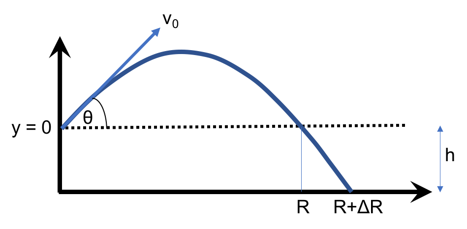
Fig. 3 A projectile is fired from some initial height \(h\) above the ground, with a new range \(R'\) compared to the simple projectile range \(R\). Our choice of where \(y=0\) is arbitrary so in this case the \(y\) coordinate of the new landing point is \(-h\). If I wanted to define the firing height as \(y=h\) then I can still solve this but the algebra becomes more challenging.

Once again we return to equation (7) but in this case we set \(y=h\) where \(h\) is the height difference between firing and landing points (positive \(h\) means landing point is higher than firing point). Thus

\[\begin{align*} h &= x\tan\theta - \dfrac{gx^2}{2v_{0}^2\cos^2\theta}\\ 0 &= x^2 - \dfrac{2v_{0}^2\sin\theta\cos\theta x}{g} + \dfrac{2v_{0}^2\cos^2\theta h}{g} \end{align*}\]

which has been rearranged into the quadratic form with \(a=1\), \(b=-\dfrac{2v_{0}^2\sin\theta\cos\theta}{g}\) and \(c=\dfrac{2v_{0}^2\cos^2\theta h}{g}\).

Solving the quadratic and taking only the positive root of the square root term (negative root gives the solution behind the firing point) is

\[\begin{align*} R' = R+\Delta R &= \dfrac{1}{2}\left[\dfrac{2v_{0}^2\sin\theta\cos\theta}{g}+\left(\dfrac{4v_{0}^4\sin^2\theta\cos^2\theta}{g^2}+\dfrac{8v_0^2\cos^2\theta h}{g}\right)^{\frac{1}{2}}\right]\\ &= \dfrac{1}{2}\left[\dfrac{2v_{0}^2\sin\theta\cos\theta}{g}+\left(\dfrac{4v_{0}^2\cos^2\theta}{g^2}\left(v_0^2\sin^2\theta+2gh\right)\right)^{\frac{1}{2}}\right]\\ &= \dfrac{1}{2}\left[\dfrac{2v_{0}^2\sin\theta\cos\theta}{g}+\dfrac{2v_{0}\cos\theta}{g}\left(v_0^2\sin^2\theta+2gh\right)^{\frac{1}{2}}\right]\\ &= \dfrac{v_0 \cos\theta}{g}\left[v_0 \sin\theta + \left(v_0^2\sin^2\theta+2gh\right)^{\frac{1}{2}}\right] \end{align*}\]

This equation is certainly more complicated than the earlier case where \(h=0\) (equation (12)) but this is a more general equation that can be used for any landing height. As a useful test you should set \(h=0\) in the above equation to show that it reduces to the form you expect for a system with the same firing and landing height.

Note

Even though I have presented this as a separate scenario, hopefully you have spotted that this is incredibly similar to the coconut example from earlier. And so it should be but in this case we are relaxing the constraint that \(h\geq0\) because the target could now be lower than the cannon.

In fact this is the solution to the question posed very early in the coconut example. If the cannon has a height of \(h_\text{cannon}\) and the coconut is on a post of height \(h_\text{post}\) then we can simplify this by taking the difference and reducing the system to the simple case of firing from ground height and trying to hit a coconut on a post of height \((h=h_\text{post}-h_\text{cannon})\).

Sloping Ramp

In this final section we are going to think about generalising the scenario further and asking ourselves why were castles built on top of hills? There is certainly the argument that climbing a hill is tiring, but by making some approximations to model the shape of a hill we can see how an upward slope changes the range of a projectile compared to an upward slope or firing on a level plane.

We are going to only consider the most simple model for a hill which is a straight line with some constant gradient. If you wanted to you can do the same process as we are about to see but use a different expression for the hill.

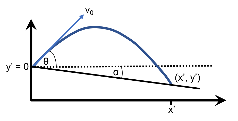
Fig. 4 Firing a projectile down a ramp inclined at an angle \(\alpha\) with respect to the horizontal, where a positive \(\alpha\) indicates an upwards sloping ramp. Care should be taken to note that the firing angle \(\theta\) is defined with respect to the horizontal, and not to the surface of the ramp. The new landing coordinates are \((x',y')\).

Projectile Range

In this situation we once again consider the intersection between the parabolic curve and the landing ‘line’. In section Launchpoint \(y\neq0\) we used the simple expression \(y=h\) but in the case of a sloping ramp we must use the equation of a straight line expressed in terms of the angle of the ramp, such that

\[\begin{align*} x'\tan\alpha &= x'\tan\theta - \dfrac{gx'^2}{2v_0^2\cos^2\theta} \end{align*}\]

where \(x'\) is the \(x\)-coordinate of the landing point on the ramp and \(\alpha\) is the slope angle. Thus

(14)\[\begin{split}\dfrac{gx'}{2v_0^2\cos^2\theta} &= \tan\theta - \tan\alpha\nonumber\\ x' &= \dfrac{2v_0^2}{g}\left(\cos^2\theta\tan\theta - \cos^2\theta\tan\alpha\right)\nonumber\\ &= \dfrac{2v_0^2}{g}\left(\sin\theta\cos\theta - \cos^2\theta\tan\alpha\right)\end{split}\]

It is worth reiterating that this expression is for the horizontal coordinate of the landing point and not the length down the ramp. However this length \(L\) can easily be found from trigonometry

(15)\[\begin{split}L &= \dfrac{x'}{\cos\alpha}\nonumber\\ &= \dfrac{2v_0^2}{g\cos\alpha}\left(\sin\theta\cos\theta - \cos^2\theta\dfrac{\sin\alpha}{\cos\alpha}\right)\nonumber\\ &= \dfrac{2v_0^2\cos\theta}{g\cos\alpha}\left(\dfrac{\sin\theta\cos\alpha - \cos\theta\sin\alpha}{\cos\alpha}\right)\nonumber\\ &= \dfrac{2v_0^2\cos\theta}{g\cos^2\alpha}\left[\sin(\theta - \alpha)\right]\end{split}\]

A (double) sensibility check can be performed here as both equations (14) and (15) should reduce to the range equation (equation (12)) when the angle of the slope \(\alpha\) is zero.

Angle for Maximum Range

Determining the angle for maximum range requires us to look for a stationary point in the function \(x'(\theta)\) or \(L(\theta)\). We are able to use either equation (14) or (15) as they both describe the same landing point, and so in this case we will (somewhat arbitrarily) work with equation (15).

\[\begin{align*} \dfrac{\mathrm{d}L}{\mathrm{d}\theta} = 0 &= \dfrac{2v_0^2}{g\cos^2\alpha}\,\dfrac{\mathrm{d}}{\mathrm{d}\theta}\left((\sin[\theta-\alpha]\cos\theta\right)\\ &= \dfrac{2v_0^2}{g\cos^2\alpha}\,\left(\cos\theta\cos[\theta-\alpha]-\sin\theta\sin[\theta-\alpha]\right)\\ &= \dfrac{2v_0^2}{g\cos^2\alpha}\,\cos\left(\alpha-2\theta\right) \end{align*}\]

As the fraction term does not equal zero we find

\[\begin{align*} 0&= \cos\left(\alpha-2\theta_{\text{max}}\right)\\ \therefore \alpha-2\theta_{\text{max}} &= \cos^{-1}(0)\\ \therefore \theta_{\text{max}} &= \dfrac{\alpha}{2} - \frac{\pi}{2}\left(n -\dfrac{1}{2}\right) = \frac{\alpha}{2}+\frac{\pi}{4} \end{align*}\]

where \(n\) is any integer. We only require the first solution, i.e. \(n=0\) which gives us the final expression. You can perform another sensibility check by seeing what happens when \(\alpha=0\), i.e the flat surface situation.

Substituting this value for \(\theta_\text{max}\) into equation (15) will give the maximum distance down the ramp when fired at \(\theta_{\text{max}}\);

\[\begin{align*} L_{\text{max}} &= \dfrac{v_0^2}{g\cos^2\alpha}\left[\frac{1}{2}\left(\cos(2\alpha)-\sin(\alpha)\right)\right] \end{align*}\]

Lecture Questions

Question 1

Question

A resident life mentor sees a water-filled balloon fall vertically past their window. Having lightning reflexes, they observe that the balloon took \(0.15\text{ sec}\) to pass from the top to bottom of the \(2\text{ m}\) high window.

Assuming that the balloon was released from rest, how high above the bottom of the window was the cheeky fresher who dropped the balloon?

[Not a projectile motion question per se, but good to get the brain working.]

Hint

Although the balloon is being released from rest, this corresponds to the top of the building and not at the top of the window.

Start this by drawing a diagram and label all the different distances and corresponding velocities (i.e. velocity at top of window and at bottom of window.).

Solution

Firstly we shall assume negligible air resistance. It’s not stated in the question but is a reasonable assumption to make, plus the question is pretty much unsolvable with the little information we are given.

Start with some definitions. The distance from the drop point and the top of the window is \(h\), height of window is \(h_w\), and the velocities of the balloon at the top and bottom of the window are \(v_t\) and \(v_b\) respectively. So we use the information about the window to find the velocity of the balloon just as it appears in view.

\[\begin{align*} h_w &= v_tt+\frac{gt^2}{2}\\ \therefore v_t &= \frac{h_w}{t}-\frac{gt}{2} \left[\approx 12.6\text{ m s}^{-1}\right] \end{align*}\]

Next we know the acceleration and the `final’ velocity (i.e. \(v_t\)) so we can determine \(h\):

\[\begin{align*} v_t^2 &= \cancelto{0}{v_0^2}+2ah\\ \therefore h &= \frac{v_t^2}{2g}\\ &= \frac{1}{2g}\left(\frac{h_w}{t}-\frac{gt}{2}\right)^2\\ &= \frac{12.6^2}{2\times9.8} \approx 8.1\text{ m} \end{align*}\]

Final step is from reading the question carefully. We are asked for the distance between the bottom of the window and the release point, which is \(8.1 + 2 = 10.1\text{ m }\).

Question 2

Question

A baseball is hit out of the stadium and is observed to pass over the stands, \(120.0\text{ m}\) from the home plate (i.e. where the batter stands), at a height of \(15.0\text{ m}\). The ball leaves the bat at an angle of \(45^\circ\) to the horizontal and is \(1.2\text{ m}\) above the ground when struck. If air resistance can be ignored, what is the minimum initial speed of the ball?

Hint

The temptation here is to set the maximum height of the projectile equal to the height of the stands, but the question isn’t asking for that. It turns out that the top of the projectile does not align with the top of the stands.

Solution

What we need to do is find the velocity or velocities that correspond to the ball hitting the top of the stand either on the upward path (between bat and maximum height), or on the downward.

There are two possible ways to solve this. One is to use the modified equations that take into account the non-zero starting height. The alternative approach that I’ll just is to simply redefine my origin as the ball-bat collision point, meaning that the reduced height of the stand is \(h'=15-1.2=13.8\text{ m}\). The value for \(x\) remains unchanged at \(x=120.0\text{ m}\).

We now use the simple equation for a projectile (no modifications for height or angle) and rearrange for \(v_0\), i.e.

\[\begin{align*} h' &= x\tan\theta - \frac{gx^2}{2v_0^2\cos^2\theta}\\ v_0^2 &= \frac{gx^2}{2\cos^2\theta\left(x\tan\theta-h'\right)}\\ &= \frac{gx^2}{(x-h')}\\ \therefore v_0 &= \pm\frac{\sqrt{g}x}{\sqrt{x-h'}} \approx 36.5\text{ m s}^{-1} \end{align*}\]

There’s only one solution that makes sense with our physical system, i.e. the positive square root. If you were to plot the projectile path with this initial velocity you’d see that the ball hits the top of the stands on the downward part of the path. This means the velocity found is the minimum velocity asked for it the question - any larger velocity will cause the ball to go above the stand even on the downward trajectory.

Question 3

Question

A perfectly elastic ball is thrown against a house, bounces back over the head of the thrower and lands on the ground. When it leaves the thrower’s hand, the ball is \(2.0\text{ m}\) above the ground and \(4.0\text{ m}\) from the wall, and has \(v_{0x} = v_{0y} = 10\text{ m s}^{-1}\). How far behind the thrower does the ball hit the ground?

Hint

Draw a diagram (of course!) but include two different paths. One showing the actual path of the ball bouncing off the wall, and another showing the path the ball would take if the wall was not in the way.

Solution

The solution to this problem requires some conceptual insight (aka a trick) regarding an elastic collision in terms of vectors. The details of the trick are below but the short answer is that the path of the ball still follows a parabola but at the wall the x-direction is reversed - think of it like drawing the parabolic path then placing a mirror on the wall.

Recognising this we then only need to find the range of a standard projectile from a non-zero height, and then subtract twice the person-wall distance. We also need to recognise that while the launch angle is not explicitly stated we know it is \(45^{\circ}\) because the horizontal and vertical components of the launch velocity are equal.

Start from the equation of a projectile from a non-zero starting point, i.e.

\[\begin{align*} h &= x\tan\theta - \dfrac{gx^2}{2v_{0}^2\cos^2\theta}\\ \therefore R &= \dfrac{v_0 \cos\theta}{g}\left[v_0 \sin\theta + \left(v_0^2\sin^2\theta-2gh\right)^{\frac{1}{2}}\right] \end{align*}\]

where \(h=2\), \(\theta=45^\circ\) and \(v_0=\sqrt{v_x^2+v_y^2}=\sqrt{10^2+10^2}=10\sqrt{2}\).

Plugging in these numbers gives

\[\begin{align*} R &= \frac{10{\sqrt{2}}}{g{\sqrt{2}}} \left[\frac{10{\sqrt{2}}}{{\sqrt{2}}} + \left(\frac{100\times {2}}{{2}}-2\times g\times 2\right)^{\frac{1}{2}}\right]\\ &= \frac{10}{g} \left[10 + \left(100-5g\right)^{\frac{1}{2}}\right]\\ &\approx 22.23 \end{align*}\]

and so the distance the ball lands behind the person is \(14.2\text{ m}\).

Although it’s not necessary it’s never a bad thing to do a sense check and I’ll do this with the range equation for a simple projectile.

\[\begin{align*} R_\text{simple} &= \dfrac{v_{0}^{2}\sin2\theta}{g}\\ &= \frac{200}{g}\approx 20.4 \end{align*}\]

The range we found earlier (\(22.2\text{ m}\)) should be larger than the simple projectile, which is indeed the case here. So while this doesn’t show that the answer to the original question is correct, it is at least reasonable compared to a more idealised case.

Explaining the ‘trick’ It’s not a trick per se but needs us to understand something about momentum in vector form. Immediately before the collision the ball has a momentum that can be resolved into \(x\) and \(y\) components. Let us define positive \(x\) in the direction from the person to the wall, and positive \(y\) as up from the ground.

When the ball hits the wall the horizontal component of momentum inverts in direction but does not change in magnitude (because it is inelastic), which is what gives us this `mirror’ effect I mentioned before. The \(y\) component however does not change in either direction or magnitude. So care needs to be taken when describing how the collision changes the momentum - you need to think about it as a vector quantity, and then be careful about which components undergo a change or inversion.