Lecture 4 - Work, potential and conservation of energy

Lecture 4 - Work, potential and conservation of energy#

Energy is, at best, strange. As a concept it perhaps the most far-reaching in terms of applicability but is also one of the most difficult to define completely and succinctly. We explain it in terms of different units, with different equations and models, and try to use general defining statements such as energy being something we ‘pay’ in order to get things done. One particular attempt that I like is from A. P. French (1971) who claimed that

Energy is the universal currency that exists in apparently countless denominations; and physical processes represent a conversion from one denomination to another.

But none of these truly define what energy is. But thankfully this should not be regarded as an issue; Kramer once reflected in a symposium that

The most important and most fruitful concepts are those to which it is impossible to attach a well-defined meaning.

Having a well-defined meaning of energy is less important and useful compared to how we consider the transformation of energy. We cannot define energy in general but we can and will make heavy use of the fact that it is conserved, a statement that we will accept at face value.1

If we take the rather fluffy statement that energy is is paid to do something, then we can define the property “work” that quantifies how this paid energy transforms our system from one state to another. For the purposes of this course we will only be considering dynamical states - I leave any thermal work for the Thermal component of the module, and take the approach that any energy that is transformed into a non-dynamical form is “lost”, though we will revisit this apparent paradox of energy being both conserved and lost in the last section.

Work and kinetic energy#

In Lecture 3 we discussed how the change in the dynamics, i.e. the acceleration of a body is a result of an applied force. We are of course making the assumption here that the mass remains constant meaning we are making use of the special case of Newton’s Second Law given by equation (20).

Let us expand on this idea. We have already established that an applied force will give rise to an acceleration, but we can consider the work done when applying this force over a certain distance.

The system we will first consider is a box being pulled along the ground with some constant force $\textbf{F}$, as shown in Fig. 12.

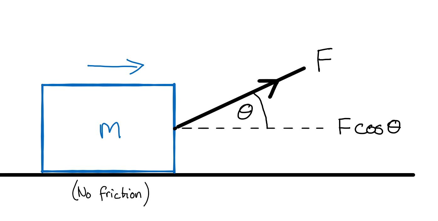
$A box dragged horizontally across a floor by a force applied at some angle $\theta$ to the horizontal. Assume there is no friction between the box and the floor.$

Fig. 12 A box dragged horizontally across a floor by a force applied at some angle $\theta$ to the horizontal. Assume there is no friction between the box and the floor.#

Assume there is no friction between the box and the ground. The work done $W$ in moving this box some distance $x$ is

\[\begin{align*} W &= F_x x\\ &= \left(F\cos\theta\right)x\\ &= \textbf{F}\cdot\textbf{x} \end{align*}\]

We need to define some terms here. $F_x$ is the horiztonal component of the force $\textbf{F}$, $\theta$ is the angle between the horizontal and the direction of $\textbf{F}$, and $\textbf{x}$ is the distance vector with magnitude $x$ and points in the horizontal direction (i.e. along the unit vector $\hat{\textbf{x}}$, such that $\textbf{x}=x\hat{\textbf{x}}$). The last line of these equations is known as the dot product or scalar product of two vectors. I am going to assume you know these as they are or will be taught in your mathematics courses.

This is the very special case in which the force remains constant over the distance $x$ so a logical next step would be to consider what happens if the force is not constant but instead is some function of $x$? We will assume for In this circumstance we make use of the special case we have just considered and think of our varying force as being the sum of lots of little displacements $\Delta x$ where the force is constant (but different) for each these small displacements.

The small amount of work done in moving the box a distance $\Delta x$ is $\Delta W$ which means

\[\Delta W = \textbf{F}\cdot\Delta \textbf{x}\]

If we make the displacements really small we can state that the total work done in moving the box from $x_1$ to $x_2$ is

(24)#\[\begin{split}W &= \lim\limits_{\Delta x \to 0} \sum_{x_1}^{x_2}\textbf{F}\cdot\Delta \textbf{x}\nonumber\\ &= \int_{x_1}^{x_2}\textbf{F}\cdot\mathrm{d}\textbf{x}\end{split}\]

Now that we have a general definition for the work done in terms of applied force and the distance over which this force is applied, let us now expand further by making use of Newton’s Second Law in the special case that the mass remains constant. The difficulty in substituting the expression $\textbf{F}=m\dfrac{\mathrm{d}\textbf{v}}{\mathrm{d}t}$ into equation (24) is that the integral is over distance but our definition of the force is a rate of change. We need to do something about the $\mathrm{d}t$.

Firstly we consider a body moving with velocity $\textbf{v}$. If a net force $\textbf{F}$ acts on the body at an angle $\theta$ to $\textbf{v}$ then we need to consider the component of the force acting in the direction of $\textbf{v}$ as we are interested in examining how this changed the magnited of $\textbf{v}$. We can write this component of the force over some small time period $\Delta t$ as

\[\begin{align*} |\textbf{F}|\cos\theta &= m \frac{|\Delta\textbf{v}|}{\Delta t}\cos\theta \end{align*}\]

where $\Delta \textbf{v}$ is the vector change in $\textbf{v}$ over $\Delta t$ and . The element of distance travelled during the time period is $\Delta\textbf{r}=\textbf{v}\Delta t$ which means the force along $\textbf{v}$ times this displacement is

(25)#\[\begin{split}|\textbf{F}||\Delta\textbf{r}|\cos\theta &= m \frac{|\Delta\textbf{v}|}{\Delta t}\cos\theta\, |\Delta\textbf{r}|\nonumber\\ &= m \frac{|\Delta\textbf{v}|}{\Delta t}\cos\theta \,|\textbf{v}|\,\Delta t\nonumber\\ &= m |\textbf{v}||\Delta\textbf{v}|\cos\theta\nonumber\\ \therefore \textbf{F}\cdot\Delta\textbf{r} &= m\left(\textbf{v}\cdot\Delta\textbf{v}\right)\end{split}\]

To simplify the right hand side of this expression we make use of a useful trick. Consider the quantity $\textbf{v}\cdot\textbf{v}$ which is a scalar of magnitude $v^2$. So if

\[\begin{align*} v^2 &= \textbf{v}\cdot\textbf{v}\\ \end{align*}\]

then the product rule of differentiation gives

\[\begin{align*} \Delta(v^2) &= \Delta\textbf{v}\cdot\textbf{v} + \textbf{v}\cdot\Delta\textbf{v}\\ &= 2\textbf{v}\cdot\Delta\textbf{v}\\ \therefore \textbf{v}\cdot\Delta\textbf{v} &= \frac{1}{2}\left(\Delta v\right)^2 \end{align*}\]

Substition of this final expression into equation (25) to find

\[\begin{align*} \textbf{F}\cdot\Delta\textbf{x} &= \frac{1}{2}m\left(\Delta v\right)^2 \end{align*}\]

and therefore the work is

(26)#\[W = \int_{x_1}^{x_2} \textbf{F}\cdot\Delta\textbf{x} = \frac{1}{2}mv_2^2 - \frac{1}{2}mv_1^2\]

If we impose the condition that the body was starting from rest at the initial position $x_1$ then we find that the work done in moving a body a distance $x$ is equal to $\frac{mv^2}{2}$, otherwise known as the kinetic energy.

Key point

In general terms the work done on a body is equal to the change of the kinetic energy of the same body.

Potential energy#

I am absolutely sure that you have heard of the concept of potential energy before, and will have worked with some of the associated formulae in your pre-University studies. The approach I am going to take here will hopefully give you a deeper insight into what we mean by potential energy and where the memorised equations (such as $mgh$) actually come from.

We start from our definition of the work done as the integral of the force applied over some distance, although for the sake of simplicity we are going to restrict the force to acting along the $x$ direction only. It’s worth emphasising however that the final result applies in general. If we define the kinetic energy of the body at positions $x_1$ and $x_2$ as $K_1$and $K_2$ respectively then equation (26) can be rewritten as

(27)#\[K_2 - K_1 = \int_{x_1}^{x_2} F(x)\,\mathrm{d}x\]

We now introduce an arbitrary reference point $x_0$ that allows us to make comparisons of states 1 and 2 with respect to this reference point. This allows us to rewrite the integral above as

\[\begin{align*} \int_{x_1}^{x_2} F(x)\,\mathrm{d}x &= \int_{x_0}^{x_2} F(x)\,\mathrm{d}x - \int_{x_0}^{x_1} F(x)\,\mathrm{d}x \end{align*}\]

which we can substitute into equation (27) to find

\[\begin{align*} K_2 + \left[-\int_{x_0}^{x_2} F(x)\,\mathrm{d}x\right] &= K_1 + \left[- \int_{x_0}^{x_1} F(x)\,\mathrm{d}x\right] \end{align*}\]

This allows us to define the potential energy $U(x)$ as follows to ensure that the conservation of energy between states 1 and 2 is met,

(28)#\[U(x)-U(x_0) = - \int_{x_0}^{x} F(x)\,\mathrm{d}x\]

The potential energy is defined as the negative of the work done by the force as the object moves from the reference point to the point of interest. It is quite common to set $U(x_0)=0$ as we are often more concerned with the differences in potential energy between one point and another.

Finally we can play around with equation (28) a little to get a slightly different form. We can differentiate both sides of equation (28) which gives

(29)#\[F = -\frac{\mathrm{d}U}{\mathrm{d}x}\]

or in everyday language the force is equal to the negative gradient of the potential.

You may be wondering why we have bothered to come up with yet another definition of the relationship between force and potential energy. Both of the forms are valuable theoretically but when it comes to taking measurements of a system it is often easier to measure the energy differences between two distinct states rather than measuring the forces acting over the whole path between these states. It is common in experimental physics to use a measureable property (in this case the potential energy) to inform us about another property that is difficult or impossible to measure.

Energy loss#

Throughout this chapter we have held the assumption that the energy is conserved. We are going to take a slight detour into a real world and terribly exciting physical system that seems to contradict this idea of the conservation of energy - the bouncing ball.

Consider a ball that is dropped from some initial height $h_0$. It falls to the vertically until it hits the ground at which point it then bounces and takes a vertical path up to a new height $h_1$, where $h_1<h_0$. The ball then falls again, bounces and reaches a new post-bounce height $h_2$. An example of this process is shown in Fig. 13 where the snapshots of the ball are displaced horizontally so you can see where the ball is as a function of time.

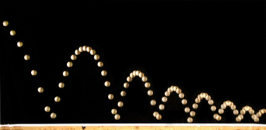
$A time-lapse image of a bouncing ball whose maximum height decreases by the same fraction between successive bounces.$

Fig. 13 A time-lapse image of a bouncing ball whose maximum height decreases by the same fraction between successive bounces.#

To understand what is happening at the impact we consider and compare the velocities of the ball immediately before ($v_i$) and immediately after ($v_f$) the bounce. We define the coefficient of restitution $C_R$ as the ratio of these velocities, i.e.

\[C_R = \frac{v_f}{v_i}\]

Despite this being a perfectly valid definition, it would be completely useless if I wanted you to calculate $C_R$ for the system shown in Fig. 13 as we do not know the velocities $v_i$ and $v_f$ for any of the bounces. Indeed these are the velocities at the instant before and after the collision so measuring them would be impossible - we would only ever be able to approximate them over some finite time period $\Delta t$.

We can however make use of the knowledge that, apart from something happening at the bounce, energy is conserved. The potential energy of before the bounce is equal to the kinetic energy immediately before the bounce, and the kinetic energy after the bounce is equal to the potential energy when the ball reaches the new height. With a little algebra magic on our definition for $C_R$ we can show

\[\begin{align*} C_R &= \frac{v_f}{v_i}\\ C_R^2 &= \frac{v_f^2}{v_i^2} = \frac{\frac{1}{2} mv_f^2}{\frac{1}{2} mv_i^2}= \frac{mgh_f}{mgh_i}\\ \therefore C_R &= \sqrt{\frac{h_f}{h_i}} \end{align*}\]

Now this is much better! We can see the maximum heights of the ball before and after a bounce which allows us to calculate $C_R$. What is even better is that we do not need to know the scale that allows us to convert from pixels to physical height as we are taking the ratio of the two values which is dimensionless.

It is pretty straightforward to do this experiment yourself. All you need is a bouncy ball, a semi-decent camera with video capability, and some way of extracting the data from the video. I did this with an iPhone camera and used the Tracker software you will use in your lab classes, and extracted the data shown in Fig. 14.

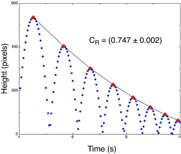
This graph shows the measured height of a ball bouncing as a function of time. The maximum points are indicated and are used to determine the coefficient of resitution from modelling the height as a function of bounce number.

Fig. 14 This graph shows the measured height of a ball bouncing as a function of time. The maximum points are indicated and are used to determine the coefficient of resitution from modelling the height as a function of bounce number.#

Rather than taking the heights before and after a single bounce I fitted a model that allowed me to determine $C_R$ based on all of the bounces recorded. Partly because this gives a more precise value for $C_R$ but also just because I could. With this experiment I found $C_R = 0.747 \pm 0.002$ which should hopefully prompt the following question: if $C_R^2$ is the ratio of the energies, should it not equal 1 because the energy is conserved? If the ball only has $86.4\%$ of the energy after the bounce compared to before, where has the $13.6\%$ gone?

Energy conserved yet lost?#

The suggestion that energy has been lost when the ball above bounces is both true and false. The apparent paradox is simple to resolve because it comes down to a case of semantics and being somewhat inaccurate with our language. When I talk about $13.4\%$ of the energy in my bouncing ball system being lost at each bounce what I should explicitly state is that $13.4\%$ of the energy is lost from the dynamic system being observed, and is transfered into some other form.

If we were to also measure the sound of the ball impacting the table, measure the vibrations in the table and the slight increase in temperature etc then we would find that the sum of all of these associated energies is equal before and after the bounce. When we talk about loss we mean from the system of interest, in this case a system in motion. The soundwaves, heat, etc produced by the bounce are now unrelated to the motion of the ball.

That is not to say that you cannot talk about energy being lost. The important point is that both you and the person you are communicating with know that you mean by lost to the system rather than lost to the universe.

Lecture Questions#

Question 1

Question

The constant forces $\textbf{F}_1 = (\hat{i} + 2\hat{j} + 3\hat{k})\text{ N}$ and $\textbf{F}_2 = (4\hat{i}-5\hat{j}-2\hat{k})\text{ N}$ act together on a particle during a displacement from position $\textbf{r}_1 = 7\hat{k}\text{ cm}$ to $\textbf{r}_2 = (20\hat{i}+15\hat{j})\text{ cm}$. Determine the work done on the particle.

Hint

Remember that both force and distance are vectors, and the work done is calculated along the direction of motion (see Fig. 12).

Solution

First calculate the net force acting on the particle:

\[\begin{align*} \textbf{F}_\text{net} &= \textbf{F}_1+\textbf{F}_2\\ &= (\hat{i} + 2\hat{j} + 3\hat{k}) + (4\hat{i}-5\hat{j}-2\hat{k})\\ &= 5\hat{i}-3\hat{j}+\hat{k} \end{align*}\]

The displacement of the particle is

\[\begin{align*} \textbf{r} &= \textbf{r}_2-\textbf{r}_1\\ &= (20\hat{i}+15\hat{j} - 7\hat{k})\text{ cm}\\ &= (0.20\hat{i}+0.15\hat{j} - 0.07\hat{k})\text{ m} \end{align*}\]

Thus the work done is

\[\begin{align*} W &= \textbf{F}\cdot\textbf{r}\\ &= \left(5\hat{i}-3\hat{j}+\hat{k}\right)\cdot\left(0.20\hat{i}+0.15\hat{j} - 0.07\hat{k}\right)\\ &= 1 - 0.45 - 0.07\\ &= 0.48\text{ J} \end{align*}\]

Question 2

Question

The potential energy of an object is given by

\[\begin{align*} U(x) &= 5x^2 - 4x^3 \end{align*}\]

where $U(x)$ is in joules and $x$ is in metres.

What is the force $F(x)$ acting on the object?
Determine the positions where the object is in equilibrium, and state whether they are stable or unstable.

Hint

Stability can be estimated graphically and determined exactly through calculus, so try both.

Solution

1

\[\begin{align*} F(x) &= -\frac{\mathrm{d}U}{\mathrm{d}x}\\ &=12x^2-10x \end{align*}\]

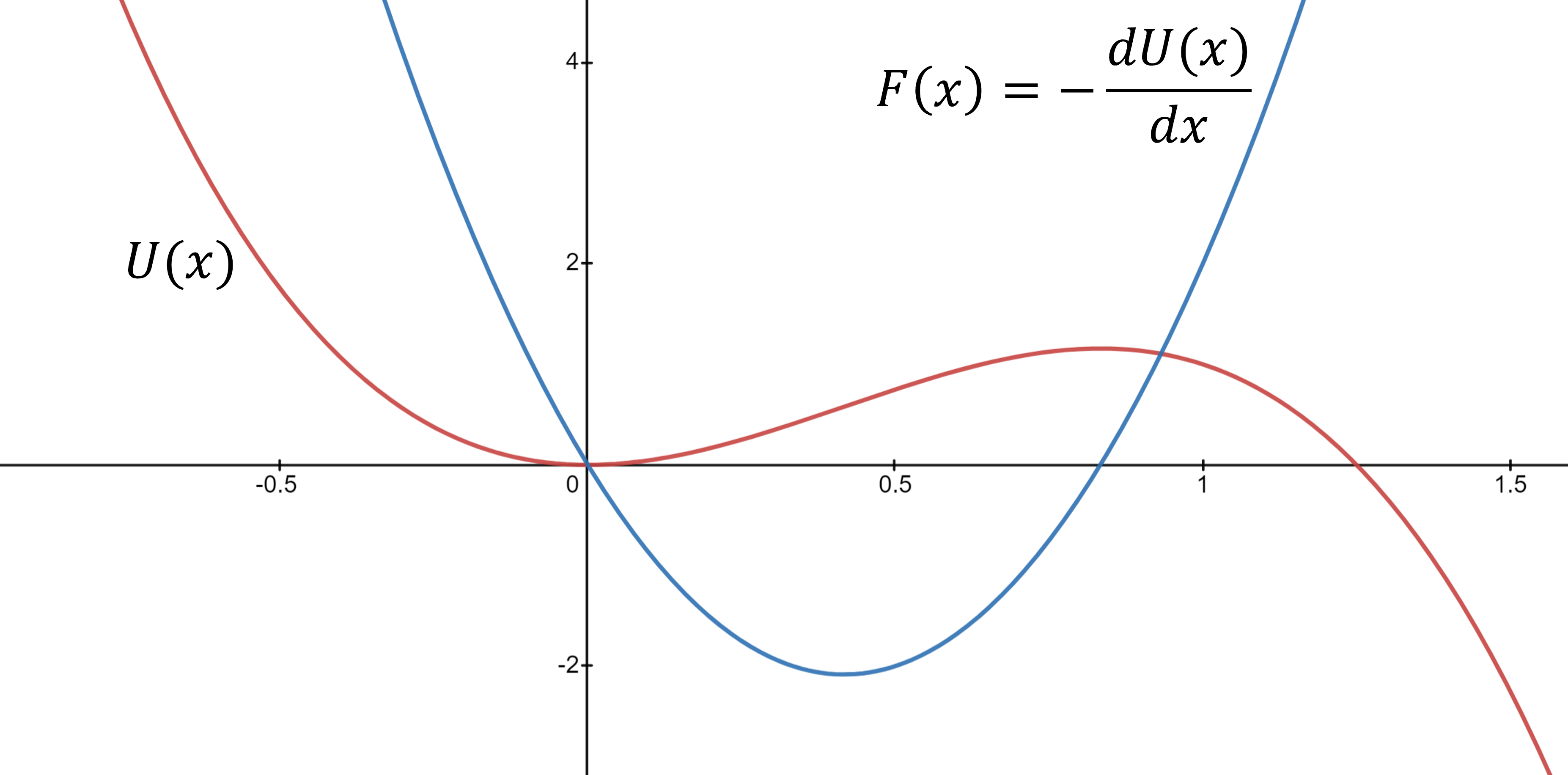
2 The condition for equilibrium is $F(x)=0$, so

\[\begin{align*} 0 &= 12x^2 - 10x = 2x(6x-5) \end{align*}\]

which has solutions $x=0$ and $x=\frac{5}{6}$.

Whether the positions are stable or not depends on whether the curvature of the equilibrium point is positive or negative, or in other words whether it is a maximum or minimum respectively. The calculus approach is to find the value for $\dfrac{\mathrm{d}F}{\mathrm{d}x}$ and evaluate it at both of the solutions found above.

For $x=0$

\[\begin{align*} \left. \frac{\mathrm{d}F}{\mathrm{d}x}\right\vert_{x=0} &= 24x-10\\ &= -10 \end{align*}\]

This is a negative value meaning that $x=0$ is a stable position.

For $x=\frac{5}{6}$

\[\begin{align*} \left. \frac{\mathrm{d}F}{\mathrm{d}x}\right\vert_{x=\frac{5}{6}} &= 24x-10\\ &= \frac{24*5}{6}-10 = +10 \end{align*}\]

This is a positive value meaning that $x=\frac{5}{6}$ is an unstable position.

The figure below shows the plots for both $U(x)$ and $F(x)$. The curve of $U(x)$ at the roots of $F(x)$ is a minimum for $x=0$ but maximum for $x=\frac{5}{6}$. Be careful with this approach however because some curves may look like they have a clear minimum or maximum but that may not be the case if you zoom in a lot - the calculus approach is safer!

Question 3

Question

A body slides down a rough plane inclined to the horizontal at $\theta=30^\circ$. If $70\%$ of the initial potential energy is dissipated during the descent, find the coefficient of sliding friction $\mu$.

Hint

A reminder that the friction force is defined as $F=\mu N$ where $N$ is the normal force.

Solution

Let the body travel a distance $s$ along the incline and down through a height $h$.

The potential energy lost $=mgh=mgs\sin\theta$.

The work done against friction $W=f_\text{k}s = \left(\mu_\text{k}mg\cos\theta\right)s$.

Thus

\[\begin{align*} \mu_\text{k}mg\cos\theta\,s &= \frac{70}{100}mgs\sin\theta\\ \therefore \mu_\text{k} &= 0.7\tan\theta\\ &= 0.404 \end{align*}\]

1: The first and perhaps most elegant general proof that energy, linear and angular momentum are conserved was published by Emmy Noether in 1918. She demonstrated that any physical system with differentiable symmetry must have corresponding conservation laws. Her work had extremely far reaching implications and set the foundations for much of the classical physics you will study, but the formal proof of Noether’s Theorem is beyond the scope of this course.

Lecture 4 - Work, potential and conservation of energy

Contents

Lecture 4 - Work, potential and conservation of energy#

Work and kinetic energy#

Potential energy#

Energy loss#

Energy conserved yet lost?#

Lecture Questions#