
Lecture 2 - Non-constant acceleration: (De)constructing suvat.#
I must confess to a tiny amount of sleight-of-hand in Lecture 1. In saying that I was going to refer to the suvat equations as kinematic equations because I wanted to change to a more standard notation I have overlooked a more fundamental point. It is this point that we will look into now.
The particular case of suvat#
In order to really think about this issue we are going to first derive the kinematic equations in such a way that we can then reassess and test our assumptions rather than focusing on the final expressions.
Many of the examples we use the suvat form of the kinematic equations for is mechanics in an every day situation. Dropping a ball, a car travelling along a road, trying to shoot a coconut off a post - all of these are a daily occurrence. For all of these simpler systems I would expect that you have worked on the assumption that the acceleration is constant, either due to gravity or because that is how the teacher set up the question for ease. Nevertheless that is where we are going to start as well.
If the acceleration has constant value \(a_0\) then we can state that
This is a very simple differential equation that we can solve by integration and imposing the initial condition that the velocity at \(t=0\) is \(v_0\) (i.e. \(v(t=0)=v_0\))
We can use the same approach to find the position as a function of time, again with the initial condition that the position at \(t=0\) is \(x_0\);
None of these derivations should be particularly groundbreaking as they are perhaps the most formal approach to deriving the suvat class of the kinematic equations. But having them set out in this way allows us to review them and see which of our steps or assumptions may cause a problem when we want to generalise our kinematic equations.
The so-called issue actually happens at the first hurdle, with equation (16). This seemingly small and unassuming equation actually imposes some significant restrictions on the use of the resulting equations. Because we are starting with the statement or assumption that the acceleration is constant then the suvat equations only apply to constant acceleration systems. I’m sure that you are generally aware of this but I think it important to stress the point; by making this assumption we are constraining the applications and physical systems that these suvat kinematic equations apply to.
But the flip side to taking this approach is that we now have a mechanism by which to generate our own kinematic equations for any system in which we know how the acceleration varies with time, that is we know an expression for \(a(t)\) which is not constant.
Key point
The suvat equations are kinematic equations for a specific condition. One way to think about them is that all suvat equations are kinematic equations, but not all kinematic equations are suvat equations.
A non-suvat example#
Let us consider a very trivial example where the acceleration of a system starts from some value \(a_0\) at \(t=0\) and then linearly increases with some constant of proportionality \(J\). This means we can define our starting equation similar to equation (16) but this time with a non-constant acceleration,
This means we can derive expressions for the velocity and position of a particle under this abstract linear acceleration condition, namely;
So here we have a nice set of kinematic equations that we could use in a similar fashion to the suvat equations you have used time and time again. But these are decidely not the suvat equations of old. And this is the critical point that I want you to take away from this example.
Key point
You always need to check the underlying assumptions of the models and tools you use. But knowing the fundamentals and derivations means you can modify the tools and create your own.
Non-constant acceleration#
So you may be asking yourself why I have spent some much time stressing that you should be very careful with the suvat equations. And you should be, because they only work under a very specific condition that actually is a rather unusual one in the real world. It is much more common that the systems you will now be dealing with in your degree have a non-constant acceleration. We are going to look at two particular situations, the simple pendulum and free fall in a fluid, plus an aside discussion on gravity that we will not formally derive but is a good mental exercise for you.
Simple pendulum#
The simple pendulum is often taught in pre-University courses but my experience is that the approach taken is similar to that we saw for projectile motion in Lecture 1. Some special points are considered, namely the equilibrium point and the maximum amplitude, but the entire path itself is not explored in depth. We are going to change that now because the simple pendulum is a really simple system to visualise that involves a non-constant acceleration.
Consider Fig. 5 that shows a pendulum of length \(l\) swinging on the orange path between two maximum amplitudes. Forgive me for jumping ahead a chapter for a brief moment but I have made use of the concept of a force, but what I have used is most definitely not new to you so let us run with it for now and leave the deeper discussions about forces until Lecture 3.
Assuming that we are playing with this pendulum on Earth but also happen to be standing in a vacuum, the only force acting on the pendulum mass is due to gravity. This means that the acceleration of the mass along the orange path, i.e. the tangential direction, is equal to the component acting in the tangential direction
as shown in Fig. 5 below. I am using the notation \(a_T(\theta)\) to be really explicit that this is the acceleration acting in the tangential direction and that it is a function of \(\theta\) and is therefore not constant.
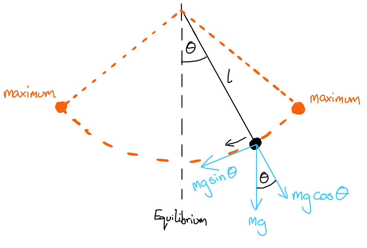
Fig. 5 A pendulum oscillating between two maximum amplitudes. The only force acting is gravity which acts downwards as indicated by the downwards arrow and has magnitude \(mg\). This force can be resolved into two components, one pointing along the length of the pendulum (with magnitude \(mg\cos\theta\)) and the other pointing in the direction of motion (with magnitude \(mg\sin\theta\)).#
But we do have a well defined function for how the acceleration varies with angular displacement so we can construct an equation that describe the motion of the mass in terms of angular displacement and time, with some constants for good measure.
We first need to switch to a more convenient coordinate system. So instead of considering the linear displacement we want to know the arc length \(s\) in terms of the displaced angle. From this we can calculate the velocity and acceleration of the mass as
We can combine this expression for \(a_T(\theta)\) with equation (17) to find
I hope that you can see that this equation that describes a simple pendulum in terms of the acceleration and displacement is very different to the suvat equations. If you tried to force the suvat equations into the system it simply wouldn’t work, which is why it is imperative to always go back to the assumptions of the system you are studying and construct the theoretical framework appropriately.
It turns out that equation (18) is a differential equation that is not easy to solve. This particular instance is a second-order nonlinear ordinary differential equation. Differential equations crop up everywhere in physics so you will see these time and time again, but for now we will leave it here as we do not need to find a solution to get the take home message regarding non-constant acceleration.
For the future
If you feel so inclined you can come back to this equation again once you have learnt a bit about differential equations and see if you can find a solution if you make use of the small angle approximation, i.e. \(\sin\theta \approx \theta.\) It should give a you familiar expression from your pre-University studies.
Free fall in a fluid#
In this section we are now going to go against the stereotype of a physicist and actually consider air resistance! Or more generally we are going to consider the case of a body moving through a fluid which includes both liquids and gases but can be extended to roughly approximate motion through more exotic states of matter such as polymer melts.
We are only going to think about a body in free fall as this simple geometry still presents a difficult setup to derive a form of a kinematic equation, namely the velocity of the body. You can extend the principles here to two or three dimensional motion, such as including air resistance in the projectile motion we have already covered in Lecture 1 but it quickly gets very hard to solve and is not necessary for this course.
So let us jump into the problem with our usual first step of defining the system, and of course we must include our labelled schematic diagram.
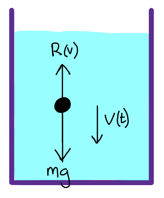
Fig. 6 An object of mass \(m\) in free fall through some fluid. The velocity of the object \(v(t)\) points downwards in the direction of gravity and there is a resistive force due to the interaction between the fluid and the moving body \(R(v)\). For this course we assume that \(R(v)\) is proportional to \(v(t)\).#
You may be questioning why I have taken the time to draw out Fig. 6 as it is a rather simple one at face value. I agree but it also allows us to pin down some definitions that will help us from making mistakes down the line. I’d like to draw your attention to the fact that the force acting downwards due to gravity is constant, whereas the resistive force \(R\) is a function of velocity. For nearly every system describing motion through a fluid this will be a positive relation meaning that increasing the velocity will increase the resistive force, but it is the exact relationship between resistive force and velocity that makes this a more challenging problem.
For the purposes of this example we are going to make the assumption that the resistive force varies linearly with velocity meaning we can state that
where the constant of proportionality \(b\) depends on the shape of the body moving through the fluid as well as the interaction between the body and fluid. Thankfully we do not need to exactly define what \(b\) is so long as we make the reasonable assumption that it remains constant.
Again I am jumping ahead a little bit but we can make use of the form of Newton’s Second Law that you have already seen (\(F=ma\)) to make a statement about the net force (and therefore net acceleration) in terms of the two component forces involved. This gives
You will see that I have used the substitution \(k=\frac{b}{m}\). It is entirely acceptable to combine multiple constants into a single constant as I have done here. Sometimes this can give some new insight into the physical meaning of the system but, more often than not, it is simply because we want to save time by only writing one letter instead of many. This efficient (read: lazy) approach is the one I have taken.
This is a differential equation which can be solved using the separation of variables method as follows
We can define this constant of integration \(c\) by considering the initial conditions of our system. As is our usual approach we can work from the assumption that the initial velocity is zero. By substituting in \(v=0\) and \(t=0\) we find \(1 = e^{-kc}\) which is only true when \(c=0\) (assuming \(k\neq 0\)). Thus
This equation shows how the velocity of a falling object in a resistive medium changes as a function of time. We can see that if \(t=0\), then \(v=0\) and when \(t=\infty\), the terminal velocity \(v_{terminal}=\frac{mg}{b}\) is obtained. Terminal velocity is reached when the gravitational force (weight) is balanced by the resistive force (eg. viscous force).
Key point
When asking whether our system is a constant or non-constant acceleration system we need to consider the net acceleration. This follows from considering the net forces that will be covered in Lecture 3.
Gravity.#
Disclaimer: We will look back at this example in a bit more detail at the very end of this course when we study gravity in Lecture 11. But this will be more for completeness and is not part of the assessed course itself.
When we entertain ourselves by studying how a mass behaves in free fall we typically make two assumptions, that there is no air resistance (although we’ve covered this in the free-fall in a fluid section and that gravity is the only force acting on the mass. This second assumption relies on the approximation that for “small distances” the gravitational force is constant or, more correctly, the change in the force over the small distance is negligible. But what happens if we wanted to calculate the time taken to impact on the Earth, or the impact velocity of a tool dropped by an astronaut undergoing a space walk on the ISS? The force due to gravity is described by
where \(G\) is the gravitational constant, \(m\) and \(M\) are the masses of the two interacting bodies, and \(r\) is the distance between the two. You may have already seen this but if you have not then worry not as we will cover it in Lecture 11. For now, just accept it as true.
We are going to now calculate the velocity the dropped tool will have when it hits the surface of the Earth, assuming no atmospheric effects and the tool is dropped from rest.
If we know the force due to gravity then we can state the acceleration due to gravity,
and we’ll define \(R_E\) as the radius of the Earth, \(h\) as the height of the ISS above the surface of the Earth, and \(r\) is the radial distance of the tool from the surface of the Earth (so \(r=0\) occurs then the tool hits the ground).
The challenging part to this problem comes when we try to link the above equation for acceleration due to gravity with the differential form of acceleration, \(\frac{\mathrm{d}v}{\mathrm{d}t}\). The acceleration due to gravity acting on the tool is not constant in time as for later times the acceleration will be larger (i.e. the tool is closer to the Earth). One approach to solving this could be to try and calculate the time taken to hit the ground and then find the velocity, but this is a bit tricky as you need an expression for how the acceleration varies in time.
Instead we can change the differential!
So now we can solve by using the expression for \(a_g\) above, rearranging and integrating,
A sense check here would be to see what happens when \(h\ll R_E\) meaning the tool is close to the surface and so the gravitational field is roughly constant. When this limit is taken you get the same result you would from the standard suvat-type kinematic equation,
This may be a rather contrived example but it has some wider reaching benefits beyond the immediate topic. The important part is that if you have a mathematical description for the force related to some physical interaction then you can use this to create lots of insightful models. For example if you knew how the force between two charged particles behaved as a function of separation between them, then you could work out the velocity of one particle if released from rest and the second particle was fixed. Or you could model the motion of charged particles through a field, which forms the basis of an experimental technique known as mass spectrometry.
Not bad for your second week at university!
Lecture Questions#
Question 1
Determine the velocity of a body falling under gravity, the resistance of air being assumed proportional to the square of the velocity.
Start with a modification to equation (19) that changes it from a \(v\) to a \(v^2\) dependence. You’ll also need the standard integral:
where \(a\) is a constant.
Start with the equation of motion
where \(k=\frac{b}{m}\) and \(V^2 = \frac{g}{k}\). This second substitution may seem a little odd but it allows us the use a standard integral
where \(a\) is a constant. Using this standard integral in our problem gives
If the body starts from rest then \(c=0\) and so
The penultimate line here actually tells us something physical about \(V\). As \(t\rightarrow\infty\) the right hand side approaches 1 meaning that \(v\rightarrow V\) - this means that \(V\) is the terminal velocity.
It is possible to derive other equations of motion such as position as function of time or velocity as a function of position. I’ll give you the answers here if you want to work through the algebra yourself.
Question 2
A body is projected upward with initial velocity \(u\) against air resistance which is assumed to be proportional to the square of velocity. Determine the height to which the body will rise.
In kinematic problems there are a number of parameters that are of interest, and we can express one in terms of another (position as a function of time, for example). Consider which two parameters are the best here.
You can use the chain rule to change from pairs of variables (position and time) to another (position and velocity).
First we define our axes such that motion occurs in the \(y\) direction and so our equation of motion is
Before we start with the algebra it’s useful to take a moment to think about where we want to end up. The question is wants us to find a height (distance in \(y\)) at the peak of motion. One approach could be to calculate the time taken for this to happen and substitute into an expression for \(y(t)\) but this is rather convoluted. We also know that at the turning point the velocity is zero so this tells us that we should aim for an expression in terms of velocity and position.
To do this we need to use the chain rule to change the variables in our equation of motion from time to position. We use
Substituting this into the equation for motion and solving gives
where \(V^2=\frac{g}{k}\) and we use the fact that \(\frac{\mathrm{d}(v^2)}{\mathrm{d}v} = 2v \implies v\mathrm{d}v = \frac{\mathrm{d}(v^2)}{2}\).
Thus
where \(c\) is the constant of integration. When \(y=0\), \(v=u\) and therefore \(c=V^2 + u^2\) and so we have
The height \(h\) to which the particle rises is found by putting \(v=0\) at \(y=h\) giving
Question 3
Under the assumption of the air resistance being proportional to the square of velocity, find the loss in kinetic energy when the body has been projected upward with velocity \(u\) and returns to the point of projection.
The previous two questions provide the two key expressions needed here. Your job is to think how to combine the two expressions.
For simplicity we’ll use the result from the two previous questions. To do this we recognise that the second half of the motion is a downward fall from rest, which is the situation for the first question but we also know the height that the object falls from the second question. In other words, we substitute the expression for \(h\) from question 2 into \(v(y)\) from question 1.
The loss of kinetic energy is \(\frac{1}{2}mu^2 - \frac{1}{2}mv^2\) so