Lecture 6 - Conservation of momentum in 2D

Lecture 6 - Conservation of momentum in 2D#

Elastic collisions in 2D - resolving method#

You will be pleased to know that we have already seen the physics we need to work with elastic collisions in two (and three) dimensions.

The hardest part, and in my experience the part that usually causes some students to trip up, is recognising that having more than one dimension means we need to think about the orthogonal components for any vector quantities involved.

Let us pick apart the last part of the paragraph above. We saw in the one dimensional elastic collision case that we make use of both the conservation of energy and conservation of momentum to find the final velocities of the two impacting bodies. The two dimensional case uses exactly the same concepts but it is important to be aware that because momentum is a vector quantity we need to resolve it into the two orthogonal components and use conservation of momentum twice, once for each component, whereas energy is a scalar quantity so we can only use this principle once.

A worked example will help clarify this and demonstrate the process of solving problems involving elastic collisions in two dimensions. In Fig. 18 a body of mass $m_1$ is moving with velocity $v_{1i}$ along the $x$-axis. It collides with a stationary body of mass $m_2$. After the collision the first body moves with a new velocity $v_{1f}$ in a straight line at an angle $\theta$ to the $x$-axis. Similarly the second body moves with velocity $v_{2f}$ at an angle $\phi$ below the $x$-axis.

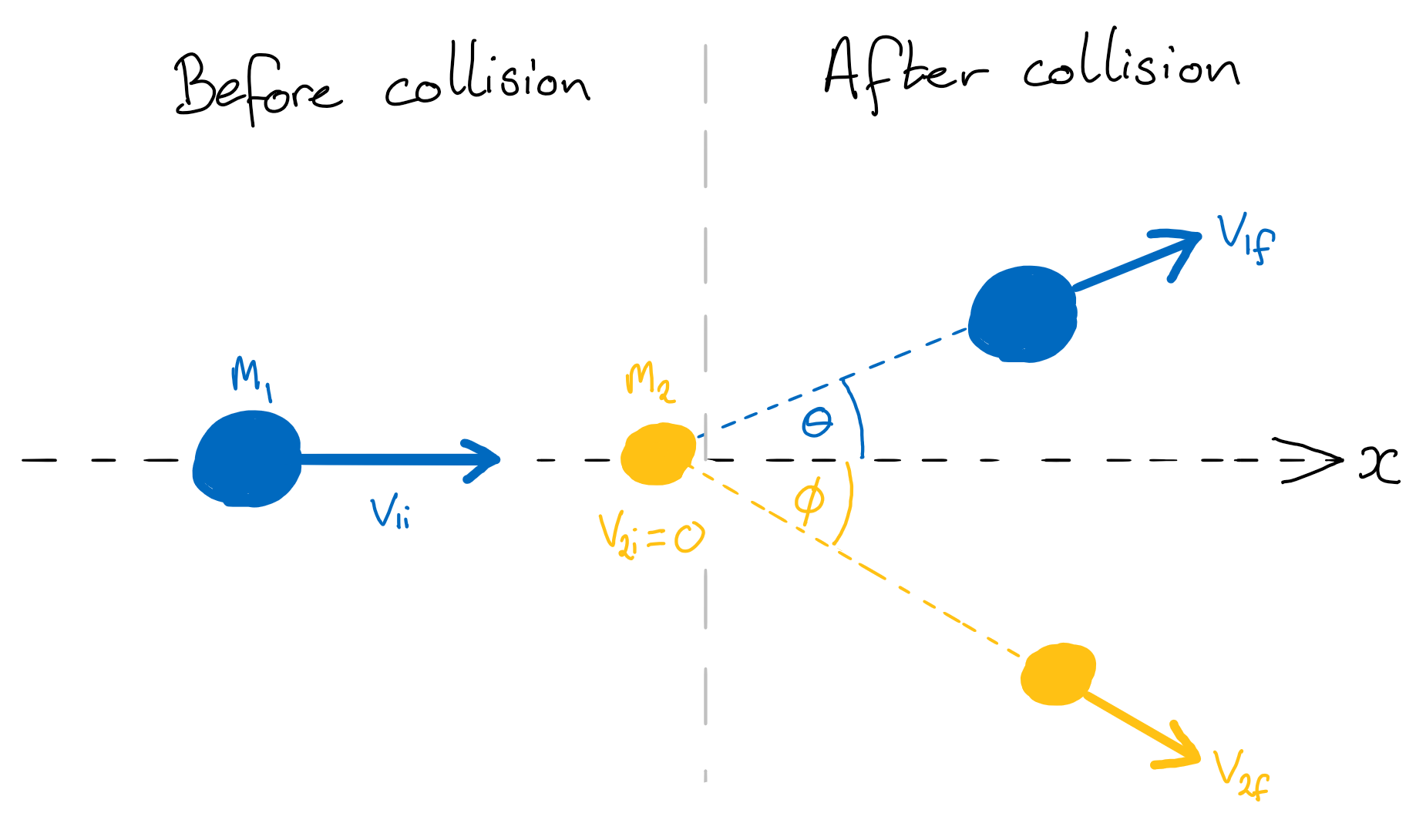
Schematic of two masses colliding. One mass initially moves along the $x$-axis and the other is stationary. After the collision the two masses move in a straight line at different angles with respect to the $x$-axis and have different velocities.

Fig. 18 Schematic of two masses colliding. One mass initially moves along the $x$-axis and the other is stationary. After the collision the two masses move in a straight line at different angles with respect to the $x$-axis and have different velocities.#

Let us start with the simplest step which is defining the total energy before and after the collision,

(40)#\[\begin{split}KE_{\text{before}} &= KE_{\text{after}}\nonumber\\ \therefore \frac{m_1v_{1i}^2}{2} + 0 &= \frac{m_1v_{1f}^2}{2} + \frac{m_2v_{2f}^2}{2}\nonumber\\ \text{or} \,\, m_1v_{1i}^2 &= m_1v_{1f}^2 + m_2v_{2f}^2\end{split}\]

Next we will consider the conservation of momentum in terms of the $y$-components before and after the collision. As body 1 is initially only moving along the $x$-axis it has no initial component of momentum in the $y$-direction, and body 2 is stationary so has no momentum whatsoever. After the collision we can make use of some simple trigonometry to define the vertical components of velocity for both bodies which leads to

(41)#\[0 = m_1v_{1f}\sin\theta - m_2v_{2f}\sin\phi\]

The final relationship we need is found by considering the conservation of momentum in the $x$-direction. We note that body 1 is moving in the $x$-direction initially which gives

(42)#\[m_1v_{1i} = m_1v_{1f}\cos\theta + m_2v_{2f}\cos\phi\]

Before we start manipulating these three equations to find expressions for $v_{1f}$ and $v_{2f}$ I want to highlight a small but really important point. In equation (42) the two terms on the right hand side are added together whereas in (41) we a calculating the difference. This minus sign in equation (41) is necessary because the vertical components of momentum are in opposite directions for the two bodies.

In terms of Fig. 18 the vertical component for body 1 is upwards (positive $y$) whereas body 2 is downwards. This is in contrast to the horizontal components of momentum for both bodies 1 and 2 after the collision - they are both moving to the right (positive $x$) and therefore we must add them together.

Great. Time for some algebra.

Equation (40) has velocity squared terms whereas equations (41) and (42) are linear with velocities. If I want to start combining equations then having these velocities to the same power means I can make some substitutions, but taking the square-root of equation (40) looks messy. So one technique I am going to use is squaring the other equations to get my velocity squared terms, and will sort out the extra terms (such as masses being squared) further down the line.

Let us square equations (41) and (42) to find respectively

(43)#\[0 = m_1^2v_{1f}^2\sin^2\theta + m_2^2v_{2f}^2\sin^2\phi - 2m_1m_2v_{1f}v_{2f}\sin\theta\sin\phi\]

(44)#\[m_1^2v_{1i}^2 = m_1^2v_{1f}^2\cos^2\theta + m_2v_{2f}^2\cos^2\phi + 2m_1m_2v_{1f}v_{2f}\cos\theta\cos\phi\]

These two equations look pretty daunting but by being careful in how I write out the equations on the page I can see some similarities between terms on the right hand sides. They both share a number of similarities, namely that $\sin$ in (43) becomes $\cos$ in (44). I also notice that there are $\sin^2$ and $\cos^2$ terms which is a major flag to me - I may be able to utilise some trigonometric identities to simplify.

Hopefully you are all familiar with the identity $\sin^2\theta + \cos^2\theta = 1$. If I add equations (43) and (44) together I can make use of this identity to find

\[\begin{align*} m_1^2v_{1i}^2 &= m_1^2v_{1f}^2 + m_2^2v_{2f}^2 +2m_1m_2v_{1f}v_{2f}\left(\cos\theta\cos\phi - \sin\theta\sin\phi\right) \end{align*}\]

We now make use of another trigonometric identity, in this case $\cos A \cos B - \sin A \sin B = \cos\left(A + B\right)$ to find

(45)#\[\begin{split}m_1^2v_{1i}^2 &= m_1^2v_{1f}^2 + m_2^2v_{2f}^2 +2m_1m_2v_{1f}v_{2f}\cos\left(\theta + \phi\right)\\ \bigg[ v_{1i} &= \sqrt{v_{1f}^2 +\left(\frac{m_2}{m_1}\right)^2 v_{2f}^2 + \frac{2m_2v_{1f}v_{2f}}{m_1} \cos\left(\theta + \phi\right)} \bigg] \end{split}\]

From here you could take a rearranged form of equation (40) that expresses one of the final velocities in terms of the other parameters, then substitute that into the above to only include the final velocity of one body, however this sort of algeabraic manipulation could go on for quite some time…

When does the algebra stop??#

You can breathe a collective sigh of relief because I’m going to stop with the algebra here. I’ve ended up finding an expression that contains all of the possible parameters for our system, so we can use this to find a single unknown if we know the other parameters.

But I want to emphasise a key point here that can save you a lot of time in the future. I have one equation that utilises the conservation of energy and two for the components of momentum, and the rest is just flexing some algebra muscles to get different forms of the momentum equations that may be useful.

Always highlight what you are being asked to find and what you already know. Although I have made use of all the equations that describe the momentum and energy of the system I would be wasting time if the question at hand asked me to find the initial velocity but I already know the masses and final velocities of both bodies. In this case I would just plug the numbers into equation (40). Simples.

I will need to make use of more equations, perhaps of different forms such as equations (43) - (45), when I have more than one unknown variable. Remember that we need as many simultaneous equations are there are unknown variables if we want to solve for each unknown.

Elastic collisions in 2D - vector method#

There is a much faster but somewhat more challenging method that could be used when working with two dimensional collisions, and that is to make use of the fact that the momenta are vectors. This means we can use techniques in vector mathematics that will allow us to ‘bypass’ the resolving into horizontal and vertical components steps. Actually the vector method still uses the horizontal and vertical components but does so in a much more condensed and efficient way.

In vector form our conservation of momentum is

\[\begin{align*} \textbf{p}_{1i} &= \textbf{p}_{1f} + \textbf{p}_{2f}\\ |\textbf{p}_{1i}|\hat{\textbf{i}}&= |\textbf{p}_{1f}|\cos\theta \hat{\textbf{i}} +|\textbf{p}_{1f}|\sin\theta \hat{\textbf{j}} +|\textbf{p}_{2f}|\cos\phi \hat{\textbf{i}} -|\textbf{p}_{2f}|\sin\phi \hat{\textbf{j}}\\ &= \left(|\textbf{p}_{1f}|\cos\theta + |\textbf{p}_{2f}|\cos\phi\right)\hat{\textbf{i}} + \left(|\textbf{p}_{1f}|\sin\theta -|\textbf{p}_{2f}|\sin\phi\right) \hat{\textbf{j}} \end{align*}\]

In column vector form it is a little easier to see why this is a much more compact method

\[\begin{align*} \left( \begin{array}{c} |\textbf{p}_{1i}|\\ 0\\ \end{array} \right) &= \left( \begin{array}{c} |\textbf{p}_{1f}|\cos\theta + |\textbf{p}_{2f}|\cos\phi\\ |\textbf{p}_{1f}|\sin\theta - |\textbf{p}_{2f}|\sin\phi\\ \end{array} \right) \end{align*}\]

where we can solve “along the rows” as separate equations.

Lecture Questions#

Question 1

Question

A red car of mass $1100\text{ kg}$ and a green car of mass $1300\text{ kg}$ collide (without injury) at a cross junction. Just before the collision the red car was travelling due east at $34\text{ m s}^{-1}$ and the green car was travelling due north at $15\text{ m s}^{-1}$. After the collision the two cars remain joined together and skid with locked wheels (meaning no more drive from the tyres). What is the direction of the skid?

Hint

This problem is much easier if you think about the centre of mass of the system, as one unique property of this is that the velocity of the centre of mass remains constant before and after a collision.

Solution

The final velocity of the joined cars coincides with the final velocity of the centre of mass which in turn is the same as the initial velocity of the centre of mass. Thus

\[\begin{align*} \textbf{v}_{CM} &= \frac{m_{\text{red}}\textbf{v}_{\text{red}}+m_{\text{green}}\textbf{v}_{\text{green}}}{m_{\text{red}}+m_{\text{green}}} \end{align*}\]

Aligning our axes such that the $x$ axis is due east and $y$ is due north, the initial velocity of the red car has no $y$ component and similarly the velocity of the green car has no $x$ component. Resolving the centre of mass velocity into $x$ and $y$ components gives

\[\begin{align*} v_{CM,x}&=\frac{m_{\text{red}}{v}_{\text{red}}}{m_{\text{red}}+m_{\text{green}}} = 16\text{ m s}^{-1}\\ v_{CM,y}&=\frac{m_{\text{green}}{v}_{\text{green}}}{m_{\text{red}}+m_{\text{green}}} = 8.1\text{ m s}^{-1} \end{align*}\]

The angle can be found as the angle between these two components, i.e.

\[\begin{align*} \tan\theta&= \frac{v_{CM,y}}{v_{CM,x}}\\ &=0.51\\ \therefore \theta &= 27^{\circ} \end{align*}\]

measured anticlockwise from the positive $x$ axis.

Question 2

Question

In an atomic collision or “scattering” experiment, a helium ion of mass $m_{\text{He}} = 4.0\text{ a.m.u}$ and velocity $v_{\text{He}}=1200\text{ m s}^{-1}$ collides with an oxygen ($\text{O}_2$) molecule of mass $m_{\text{O}_2}=32\text{ a.m.u}$ which is initially at rest. The helium ion exits the collision at $90^{\circ}$ from its incident direction with one quarter of its original kinetic energy.

What is the recoil speed of the oxygen molecule?
What fraction of the total kinetic energy is lost during the collision?
What possible mechanisms could explain this ``loss’’ of energy, given the usual `suspects’ are absent at the atomic level?

Hint

Remember that you can define your coordinate system in the most convenient way to suit the physical system. Just so long as the rules still apply (i.e. in Cartesian coordinates the rule is that the axes are perpendicular).

Solution

1 Firstly we shall adopt the convention that a lower case letter refers to the He ion and upper case for the $\text{O}_2$, otherwise the notation gets a bit messy. We also use subscripts to indicate initial and final velocities

From the statement regarding the kinetic energy of the helium ion we know

(46)#\[\begin{split}\frac{1}{2}mv_f^2 &= \frac{1}{4}\times\frac{1}{2}mv_i^2\nonumber\\ \therefore v_f &= \frac{v_i}{2}\end{split}\]

We next align our axes such that the initial direction of the He molecule is along the positive $x$ axis and the direction of He molecule after collision is along positive $y$. Conservation of momentum applies due to the absence of any external forces, and so considering conservation of momentum along the two directions gives

\[\begin{align*} mv_i &= MV_{f,x} &\text{x component}\\ 0 &= mv_f + MV_{f,y} &\text{y component} \end{align*}\]

We know that $M=8m$ and so substituting this along with equation (46) into the above expressions for momentum gives

\[\begin{align*} V_{f,x} &= \frac{m}{M}v_i = 150\text{ m s}^{-1}\\ V_{f,y} &= -\frac{m}{M}v_f = -75\text{ m s}^{-1} \end{align*}\]

Thus the total speed of the oxygen molecule after collision is $V_f = \sqrt{V_{f,x}^2+V_{f,y}^2} = 170\text{ m s}^{-1}$.

2 The fraction of kinetic energy lost $\Delta E$ is the difference in kinetic energy before and after the collision divided by the kinetic energy before, i.e.

\[\begin{align*} \Delta E&= \frac{K_{\text{before}}-K_{\text{after}}}{K_{\text{before}}}\\ &= 1-\frac{K_{\text{after}}}{K_{\text{before}}}\\ &= 1- \frac{\frac{1}{8}mv_i^2+\frac{1}{2}MV_f^2}{\frac{1}{2}mv_i^2}\\ &= 1 - \frac{1}{4}-\frac{M}{m}\left(\frac{V_f}{v_i}\right)^2\\ &=0.59 \end{align*}\]

3 This 59% of the initial kinetic energy is lost to internal motions of the oxygen molecule, namely rotational and vibrational motion.