
Lecture 5 - Conservation of momentum in 1D#
In a similar vein to the start of Lecture 4 we find ourselves faced with a concept that is difficult to give a well-defined meaning but is nevertheless incredibly useful in classical mechanics. I have already made use of this definition earlier but it is worthwhile to restate it for emphasis.
Reminder
The momentum of a body with constant mass \(m\) moving with some velocity \(\textbf{v}\) is
where \(\textbf{p}\) is a vector quantity in the same direction as \(\textbf{v}\).
From forces to momentum - the impulse-momentum theorem#
Remember back in the section on Work where we looked at Newton’s Second Law and considered what it means to integrate this over distance? I mentioned in the footnote there that we would revisit this process but integrating over time. That time is now.
We start from equation (21) but will assume for now that the net force acting during some time interval \(\Delta t\) is constant. Thus we can derive the impulse-momentum theorem which states
where \(\textbf{J}\) is the impulse and \(\Delta \textbf{p}\) is the change in momentum. You may not have been taught about impulse prior to this but there is a good rationale why this is a useful quantity in certain circumstances.
Consider a constant force acting on an initially stationary body which will cause the body to accelerate, but an important piece of information is for how long the force is acting on the body. A \(1\text{ N}\) force acting on the body for one second gives a different final system compared to one acting on the body for 10 seconds. Now you could go back to the kinematic equations we saw in Lecture 2 to find the final velocities of both of these situations, but it is often easier to make use of the impulse-momentum theorem to directly find the change in momentum and thus the change in velocity.
For the 1 second case
whereas for the 10 second case
It’s important to note that this gives the change in velocity. A lot of problems may specify the initial or final velocity as being at rest (to simplify the problem) but it’s important you check this is valid rather than assuming it is true for all cases.
But what about the case where the net force is not constant? We get the same result albeit in through a slightly more difficult route,
Conservation of momentum#
One of the most far reaching and useful property of momentum is that is a conserved property. Once again the formal proof of Noether’s Theorem shows that conservation of momentum is necessary due to the differentiable symmetry of space, but this theorem is not necessary to learn for this course. We can however make some use of Newton’s Laws to demonstrate that momentum is indeed conserved.
If we have an isolated system of two bodies where the net force of body A acting on body B is \(\textbf{F}_{AB}\) and that of body B on A is \(\textbf{F}_{BA}\) then we can make use of Newtons Second Law to state
These two statements can be combined by making use of Newton’s Third Law:
The total momentum of this system of two bodies is \(\textbf{P}=\textbf{p}_A+\textbf{p}_B\). This means that equation (30) can be rewritten as
which is only true if \(\textbf{P}\) is constant.
Key point
The total momentum of a system is constant if the vector sum of the external forces acting on the system is zero.
Collisions in 1D#
Knowing the definition of momentum and the conservation of momentum law is all well and good but being able to apply it is much more useful. For the remainder of this chapter we are going to look at some very idealised cases in one dimension and see how the conservation of momentum can be used and how it does (or does not) apply in conjunction with the conservation of energy. As in all cases where we are only considering the idealised case there is quite a departure from the real world applications, but as ever a good foundation in the principles and dealing with idealised cases allows you to modify and expand for every more complicated and realistic situations.
The two types of idealised collisions we will explore are the perfectly elastic case and the perfectly inelastic case. It is worth stressing here that whilst kinetic energy may or may not be conserved for the different cases we will examine, the total momentum is always conserved in the absence of any external forces. A common mistake in dealing with these types of systems is assuming that kinetic energy is equal before and after the collision - if you need a reminder about the subtle nuance around energy loss then go back to the Energy Loss section for a refresher.
Perfectly elastic collisions#
An elastic collision is defined as a collision where the kinetic energy of the system is the same before and after the collision. In other words, the total kinetic energy is conserved.
Imagine we have two objects \(A\) and \(B\) with masses \(m_A\) and \(m_B\) respectively, and are travelling along the \(x\)-axis with initial velocities \(\textbf{v}_{Ai}\) and \(\textbf{v}_{Bi}\) respectively. In the event that they collide the bodies then have final velocities \(\textbf{v}_{Af}\) and \(\textbf{v}_{Bf}\) respectively. We know that the total momentum is conserved which allows us to state,
Note that the momenta and velocities in the above expressions are vectors, as they should be. It does allow us to readily expand this into a two and three dimensional system but for the sake of easier visualisation I am going to split out the magnitude and directions of the vectors. For our one dimensional case this is trivial as the direction is either positive or negative along the \(x\)-axis - anything other than this and it would not be a one dimensional system. This gives
where a negative velocity means the body is travelling in the negative \(x\) direction.
We are going to consider the four different types of system that can be constructed when we start to give different directions and relative velocities to the bodies \(A\) and \(B\). In each of the cases we are going to focus on calculating the final velocities assuming that we know the masses and initial velocities.
Moving towards each other initially
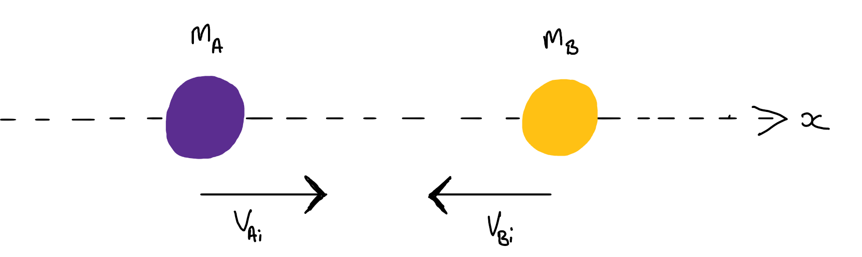
Fig. 15 Two masses \(m_1\) and \(m_2\) moving towards each other along the \(x\) axis with different velocities.#
We will be making use of equation (31) but if we are wanting to derive expressions for both of the final velocities then this equation alone is not enough. In order to solve for two variables we need two equations. We need to make use of the physics involved in an elastic collision and note that the total kinetic energy is also conserved. This means that
With some fairly straightforward algebra and making use of the completing the square method we find
Now we take the rearranged form of equation (31), namely \(m_A\left(v_{Ai}-v_{Af}\right)=m_B\left(v_{Bf}-v_{Bi}\right)\) and substitute this into equation (32) above. This then simplifies to
Taking this equation and substituting for \(v_{Bf}\) into equation (31) gives
where \(M\) is the total mass \(m_A + m_B\).
You can follow similar steps to find the following expression for \(v_{Bf}\)
Sense Check
This is a perfect opportunity for me to emphasise one of the most important yet often underrated problem solving techiques in physics. The idea behind this sense check process is to take the results you have from your derivations, in our case equations (34) and (35), and apply some specific conditions to see whether the model in the equation represents what you would expect to happen in the real world.
Take the first example of imposing the condition that \(m_A = m_B = m\). With this condition in mind our two equations become
which in words would be described as an exchange of velocities. This is much more apparent if we think about a snooker or pool situation and we say that one of the balls is initially at rest. Once the moving ball of identical mass hits the stationary ball then the initially moving one stops completely and the initially stationary ball moves off with the inital velocity of the impacting ball.
Another condition we can think about is assuming that one of the masses is significantly larger than the other. For the interest of making the interpretation easier we are going to impose the condition that \(v_{Bi}=0\), although the actual conceptual understanding we draw from this still applies if object \(B\) is initially moving.
If \(m_A\ll m_B\) then our two equations for the final velocities become
Putting this into English we would say that the little mass \(A\) bounces off the much larger mass \(B\) and goes backwards with the same velocity (remember this is an elastic collision) whereas mass \(B\) just stays still. This checks out with what we would expect for throwing a small mass at a much larger mass.
Taking the reverse condition of \(m_A\gg m_B\) we find
Translating this into the real world experience we find that the much heavier and initially moving mass just keeps going at the same speed after the collision whereas the much smaller and initially stationary mass flies off at twice the speed of the incoming large mass. Again this checks out with our expectations based on our experience of reality.
Moving away from each other at the start
The objects simply do not collide.
Nevertheless if you were to plug the values into equation (31) you would still get an `answer’ for the variable you were solving for, and generally you end up with the rather obvious results of \(v_{Ai}=v_{Af}\) and \(v_{Bi}=v_{Bf}\).
Moving in positive \(x\) direction, \(v_{Ai}> v_{Bi}\)
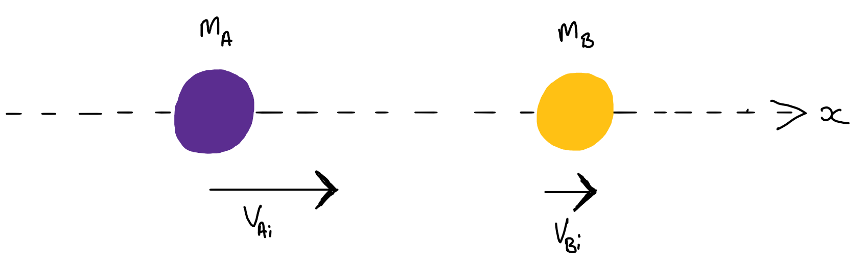
Fig. 16 Two masses \(m_1\) and \(m_2\) moving towards each other in the same direction along the \(x\) axis with different velocities. The velocity of the mass in front is less than that of the mass behind. Without this condition the masses will not collide.#
You will be pleased to know that we have already done this derivation in the first case (“Moving towards each other initially”).
We have determined, from simply looking at the system, that a collision will indeed take place so we can use the exact same result as above. The only difference here is that when we get to the stage of putting in the values for the initial velocities they will all be the same sign - in the diagram above they will all be positive but it is also applicable to the bodies moving in the negative \(x\) direction but will require \(v_{Ai} < v_{Bi}\) for a collision to occur.
Moving in positive \(x\) direction, \(v_{Ai} < v_{Bi}\)
The objects simply do not collide. Mass \(B\) is ahead and has a larger velocity, so mass \(A\) never catches up with \(B\).
Perfectly inelastic collisions#
We now move away from the elastic condition that has by definition the requirement that the total kinetic energy in conserved. In an inelastic collision the total kinetic energy is not conserved which means some of the initial energy is ‘lost’ during the collision. Although we could consider systems where a collision occurs and the two bodies move apart (i.e. considering the elastic case but with energy loss) this turns out to be somewhat complicated as we need to quantify the amount of energy lost. This is beyond what we need to do for this course so instead we will focus our attention on a specific case of inelastic collisions in which the two initially separate bodies stick together at and after the collision, and thus move as one body.
Compared to the elastic case this situation is much easier to derive. We start again by stating the conservation of momentum equation (31) but we now have a single mass \(M\) moving with velocity \(v_f\) after the collision. Thus
The final velocity is the sum of the weighted initial velocities, where the weighting is determined by what fraction of the total mass each body represents. I am going to give you three sense check conditions that you should think about and see whether the modified version of equation (36) describes what you would expect to happen in the real world.
\(m_A = m_B = m\)
\(m_A \ll m_B\)
\(m_A \gg m_B\)
Ballistic pendulum example#
A nice example is always a good way to test our understanding of a topic. In this case we are going to investigate an old method for measuring the speed of darts and bullets. In the days before high speed cameras it was not possible to measure the exit velocity of a bullet as it left the barrel using photographic or stroboscopic methods; the bullet was simply too fast to image with these techniques. Instead a system was devised in which the bullet is fired into a much larger solid block that is suspended from a rope. As the bullet strikes and is embedded in the block, the bullet + block system swings backwards to a maximum height before swinging back. By measuring the maximum height of this much heavier (and therefore much slower) bullet + block we can calculate the velocity of the bullet before impact.
There is a schematic of this experimental setup in Fig. 17.
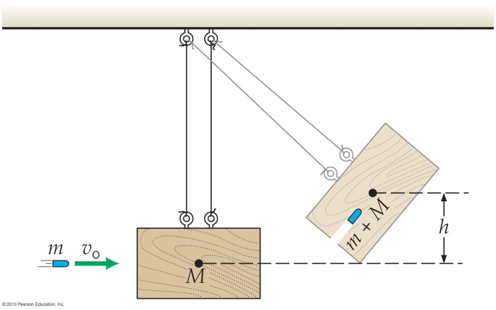
Fig. 17 Schematic of the ballistic pendulum. The block of mass \(M\) is initially at rest and the bullet of mass \(m\) and velocity \(v_0\) impacts the block. The bullet embeds into the block and the whole system swings out to some height \(h\).#
We shall start this example by first stating what physical principles apply at the different points of the process. The reason I am doing this is so we have a clear description of each step, and then we are more confident that the equations and models we apply are appropriate to each of the steps.
Let us start with the first step between the bullet leaving the barrel and immediately before striking the block. We will make the assumption that there is negligible air resistance, or alternatively we say the barrel is really close to the block, which means that the velocity remains constant up until the bullet strikes the block. More formally we can say that both energy and momentum are conserved, though this is not particularly useful here.
We now consider the collision itself. The bullet has an initial velocity and the block is stationary, but immediately after the collision the bullet + block is moving with a new velocity. It is worth stating explicitly that because this collision is inelastic there is some energy lost from the system due to the collision.
Finally after the collision the bullet + block is moving with some velocity and therefore has kinetic energy. The system swings up to a maximum height and when it reaches this stationary point all of the energy in the system is now gravitational potential energy.
It may seem really pedantic that I have gone through this first stage with a lot of words but every year so far a sizeable number of students make the incorrect assumption that the initial kinetic energy of the bullet before impact is all converted into potential energy at the maximum of the swing. My hope is that by now providing a step by step description it is more explicit that energy loss occurs and you are clear at which point it occurs during the process.
Time for some equations plus some definitions. The bullet has mass \(m\) and initial velocity \(v_0\). It impacts and embeds into a block of mass \(M\), and immediately after the impact this \(m+M\) system moves with a velocity \(v_f\).
At the collision we have already identified that energy is not conserved so it would be incorrect to say \(KE_i = KE_f\) or \(\frac{mv_0^2}{2}=\frac{\left(m+M\right)v_f^2}{2}\). What we can say is that momentum is conserved over the collision and therefore
After the collision has occured there are no processes in which energy can be lost from the system we can now make use of the conservation of energy. We can define the kinetic energy immediately after the collision in terms of \(v_f\) and thus
where \(h\) is the height of the stationary point with respect to the initial resting position of the block (see Fig. 17). We now combine equations (37) and (38) to give an expression for the initial velocity (our parameter of interest) as a function of the maximum swing height (the measurable property),
There are some limitations to this model though. It assumes that as the velocity increased more and more the height will also increase more and more. However when we think about the physical system itself we can see that the height is limited between \(0\leq h \leq 2L\) where \(L\) is the length of the rope from which the block is suspended. This value of \(2L\) corresponds to the bullet + block being at the top of the circle traced out by the swing of the system. It is sometimes easier to express the swing in terms of angle rather than change in height of the block, which is something for you to try.
Lecture Questions#
Question 1
The collision between an empty car (mass \(m\) and initial velocity \(v_i\)) and a solid barrier lasts \(0.120\text{ s}\).
Derive an expression for the average force exerted on the wall, if the velocity of the car after the collision is \(v_f\).
If the mass of the car is \(1700\text{ kg}\) and the initial and final velocities are \(13.6\text{ m s}^{-1}\) and \(-1.3\text{ m s}^{-1}\) respectively, calculate the average force on the barrier.
There are lots of parameters involved here. It can help to list the ones you know (mass, velocity and time), the ones you’re after (force), and identify any intermediate ones you may need to calculate (in this case, momentum).
1 With the \(x\) axis along the direction of the initial motion, the change in momentum is
2 Plugging in the numbers will give the force on the car by the wall
From Newton’s 3rd law the forces on the car and barrier are of equal magnitudes and opposite directions. Therefore the average force on the barrier is \(\left<F\right> = +2.11\times10^{5}\text{ N}\)
Question 2
A SuperBall, made of a rubberlike plastic, is thrown against a smooth, hard wall. The ball strikes the wall from a perpendicular direction with speed \(v\). Assuming that the collision is perfectly elastic find:
the speed of the ball after the collision.
the change in momentum of the ball.
Pay close attention to the words used in the question. In this case whether you’re asked for a scalar or a vector quantity.
1 We assume that the collision is perfectly elastic, in part because the wall is much more massive than the ball and as such the reaction force of the ball on the wall will not impart any appreciable velocity on the wall. Therefore the velocity of the ball after the is simply \(-v\).
2 If the \(x\) axis is definited in the direction of the initial motion, then the momentum before the collision is \(p_{\text{before}} = mv\) and the momentum after is \(p_{\text{after}} = -mv\). Hence the change in momentum is \(\Delta p = p_{\text{after}} - p_{\text{before}} = -2mv\).
The wall has an equal and opposite momentum change of \(+2mv\) so that the total momentum is conserved. The wall can `acquire’ this momentum without acquiring any appreciable velocity because its mass is so large, and it is attached to an even more massive building.
Question 3
An empty railway carriage of mass \(m_1 = 20\) metric tons rolling on a straight track at \(v_{1i}=5.0\text{ m s}^{-1}\) collides with a loaded stationary carriage of mass \(m_2 = 65\) metric tons. Assuming the cars bounce off each other elastically, find the velocities after the collision.
The expressions needed have already been derived above. The fact these are extended masses (carriages) rather than small coloured dots makes no difference.
Starting from equations (34) and (35) and setting \(v_{2i}=0\) we can use the values in the question to find
I have left the mass units as tons because the fractions in the above equations are a ratio of masses so the overall term is dimensionless. Always worth checking, but if in doubt convert to SI units to be on the safe side.
Question 4
Suppose that the carriages in question 3 coupled during the collision and remain locked together.
What is the velocity of the coupled carriages after the collision?
How much energy is lost during the collision?
“Coupled together” means the collision is inelastic.
1 We have a completely inelastic collision here, so from the conservation of momentum
2 The energy lost \(E\) is the difference between the final and initial kinetic energies