Lecture 9 - Rolling Motion

Disclaimer: This is by far my most favourite topic to teach in the first year Mechanics course so you will have to forgive me if I come across as overly enthusiastic in this chapter.

Rolling = translational + rotational

So far we have learnt about systems moving with linear dynamics (Lecture 1 to Lecture 6 and systems that are rotating (Lectures 7 and 8). We can now turn our attention to the more complicated but also very common in real life systems that are rotating but also have translational motion. The most obvious system that we can examine is that of a circular object (ball or cylinder) rolling down a ramp. It is obviously rotating but also moves down the ramp.

The way that we describe this rolling motion is by making heaving use of the centre of mass for the object. If we look at Fig. 26 we can see a silver disc rolling along a flat surface. The disc has two coloured markings, one at the centre of mass (in yellow) and one at the edge of the disc (in red). As you can see when the yellow and red positions are all displayed for the entire length the disc rolls along, the red position moves along a cycloid path from the flat surface to a maximum height equal to the diameter of the disc. The yellow centre of mass position however is a flat line parallel to the flat surface.

So for a rolling disc the centre of mass is moving with linear motion only, which allows us to make connections between the rotational and linear kinematics.

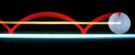
Fig. 26 A time-lapse image of a disc rolling along a horizontal surface. The centre of mass is marked and traces out a horizontal path whereas the edge of the disc (marked in red) traces a cycloid path. Thus we can use linear kinematics to describe the motion of the centre of mass.

For an object that is rolling without slipping the linear distance travelled by the centre of mass is equal to the arc length between the first and last points on the edge of the disc. A way to visualise this is to imagine applying some wet paint to the edge of the disc. If you roll it along some distance \(s\) then the paint transfered from the disc to the surface is the arc length on the disc. A schematic diagram is shown in Fig. 27.

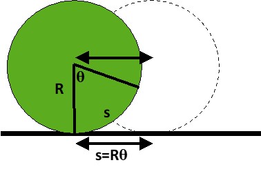
Fig. 27 A disc of radius \(R\) rolls along and rotates by some angle \(\theta\). The arc length of this is equal to the linear distance travelled along the ground.

We know that the arc length, radius and angle are all related, namely \(s=R\theta\), and we have established now that the linear distance travelled by the centre of mass is equal to the arc length, and therefore we can show that

(55)\[\begin{split}v_\text{CM} &= \frac{\mathrm{d}s}{\mathrm{d}t}\nonumber\\ &= R\frac{\mathrm{d}\theta}{\mathrm{d}t}\nonumber\\ &= R\omega\end{split}\]

and

(56)\[\begin{split} a_\text{CM} &= \frac{\mathrm{d}v_\text{CM}}{\mathrm{d}t}\nonumber\\ &= R\frac{\mathrm{d}\omega}{\mathrm{d}t}\nonumber\\ &=R\alpha\end{split}\]

I have already stated that rolling motion is the combination of translational (linear) motion and rotational motion, but now we are able to express the rotational motion in a linear form when we consider the centre of mass.

The same also applies for kinetic energy which is, as we know, fundamentally linked to the velocity of a body. For a rolling system the total kinetic energy \(K_T\) is

\[\begin{align*} K_T &= K_\text{translational} + K_\text{rotational}\\ &= \frac{1}{2}mv_\text{CM}^2 + \frac{1}{2}I\omega^2 \end{align*}\]

Let us now work through an example problem involving a cylinder rolling down an incline.

Example - Solid cylinder down a ramp

Consider a solid cylinder of mass \(m\) and radius \(r\) initially at rest on top of a ramp of height \(h\) inclined by some angle \(\theta\) to the horizontal. The cylinder is given a gentle push and begins to roll down the ramp without slipping. We want to calculate the centre of mass velocity of the cylinder at the end of the ramp.

To approach this we first assume that the system is isolated in that there is no energy lost from the mechanical system. This allows us to state that the change in gravitational potential energy must equal the total kinetic energy of the cylinder at the end of the ramp. In other words

\[\begin{align*} mgh &= \frac{1}{2}mv_\text{CM}^2 + \frac{1}{2}I\omega^2 \end{align*}\]

We next substitute for \(\omega\) using equation (55) and the moment of inertia for a solid cylinder \(I = \dfrac{1}{2}mr^2\) to find

(57)\[\begin{split}mgh &= \frac{1}{2}mv_\text{CM}^2 + \frac{1}{2}\left(\dfrac{1}{2}mr^2\right)\left(\frac{v_\text{CM}^2}{r^2}\right)\\ 2gh &= v_\text{CM}^2 + \frac{1}{2}v_\text{CM}^2\\ \therefore v_\text{CM} &= \sqrt{\frac{4gh}{3}}\end{split}\]

It is worth doing a sense check here. If we consider the more simple case of an object with mass \(m\) sliding down a frictionless incline then the centre of mass velocity of the object will be \(\sqrt{2gh}\). This is larger than the centre of mass velocity for a rolling object which checks out with our intuition: if both the rolling and sliding object start from the same height they have the same potential energy, but while the sliding object converts this all to linear kinetic energy the rolling object “shares” the energy between rotational and translational motion.

You can take this further and calculate the time taken to roll down a ramp of length \(L\), calculate the rotational velocity of the cylinder at the end of the ramp, and so on. You are now at the stage where you can start drawing on the different concepts and tools we have learned about in the previous chapters and make them work to solve whatever problem you have in front of you.

Rolling Race

Let us have a race. Imagine that we set a number of different shapes at the top of a ramp of height \(h\), and released them from rest. Which shape should reach the bottom of the incline first? The shapes we’re using are some of those we saw in Lecture 8, namely:

1. A hollow cylinder.

2. A solid cylinder.

3. A hollow sphere.

4. A solid sphere.

We have already solved this for the solid cylinder above, so we just need to modify equation (57) slightly so that it applies to the general case rather than using a specific expression for the moment of inertia for a specific shape. In other words, we want to use the general \(I=cMR^2\).

(58)\[\begin{split}mgh &= \frac{1}{2}mv_\text{CM}^2 + \frac{1}{2}\left(cmr^2\right)\left(\frac{v_\text{CM}^2}{r^2}\right)\\ mgh &= \frac{1}{2}(1+c)mv_\text{CM}^2\\ \therefore v_\text{CM} &= \sqrt{\frac{2gh}{1+c}}\end{split}\]

From this expression we can find our answer of which shape will get to the bottom first, i.e. is the one with the highest centre of mass velocity at the bottom of the ramp. The way to maximise \(v_\text{CM}\) in equation (58) is to make \(c\) smaller. So shapes with a smaller \(c\) value will reach the bottom first.

The solid sphere \(\left(c=\frac{2}{5}\right)\) finishes first, then the solid cylinder \(\left(c=\frac{1}{2}\right)\), then the hollow sphere \(\left(c=\frac{2}{3}\right)\) and finally the thin cylinder \((c=1)\).

Something else to note from equation (58) is the absence of any mass or radius terms. This means the centre of mass velocity of all solid cylinders, for example, will be the same regardless of how large or heavy they are. It only depends on the shape distribution quanitifed by \(c\).

Lecture Questions

Question 1

Question

Prove that the moment of inertia of a uniform solid sphere of mass \(M\) and radius \(R\), rotating about an axis through its centre of mass, given by \(I_{\text{CM}}\) is

\[I_{CM}=\frac{2}{5}MR^{2}\]

using the moment of inertia of a thin solid disc \(I_{disc}=\frac{1}{2}mr^{2}\) where \(m\) and \(r\) are the mass and radius of the disc respectively.

Hint

A solid sphere can be modelled as a series of concentric disc stacked vertically, going from a small disc up to the largest at the equator, then back to small again. Think of stacking a coins of increasing size then down to the smallest again.

You’ll then need to recall that

\[I_\text{sphere} = \int\mathrm{d}I_\text{disc}\]

Solution

We start by recognising that the moment of inertia of a solid sphere is the sum of the moment of inertia of many thin discs rotating about the same axis as the solid sphere, i.e.

\[\begin{align*} I_{\text{sphere}} &= \int\,\mathrm{d}I_{\text{disc}}\\ &= \frac{1}{2}\int y^2\,\mathrm{d}m \end{align*}\]

where I have aligned the axis of rotation along \(x\) and so the radius of the disc is \(y\) and thus its volume \(\mathrm{d}V = \pi y^2\,\mathrm{d}x\).

The disc and sphere are both uniform which means the density of a disc is equal to the density of the sphere, and so

\[\begin{align*} \rho = \frac{M}{V} &= \frac{\mathrm{d}m}{\mathrm{d}V}\\ \therefore \frac{M}{\frac{4}{3}\pi R^3} &= \frac{\mathrm{d}m}{\pi y^2 \mathrm{d}x}\\ \mathrm{d}m &= \frac{3M}{4\pi R^3} \pi y^2 \,\mathrm{d}x =\left(\frac{3M}{4R^3}\right)y^2\,\mathrm{d}x \end{align*}\]

We substitute this into our original equation for the moment of inertia for a sphere and find

\[\begin{align*} I_{\text{sphere}} &= \frac{1}{2}\int y^2\left(\frac{3M}{4R^3}\right)y^2\,\mathrm{d}x\\ &= \frac{3M}{8R^3}\int y^4\,\mathrm{d}x \end{align*}\]

Finally we need to express \(y\) in terms of \(x\) which we do by noting that the edge of the discs and therefore the edge of the sphere in the \(x,y\) plane can be described using the equation of a circle, i.e. \(R^2 = x^2 + y^2\) or \(y^2 = R^2 - x^2\), which yields

\[\begin{align*} I_{\text{sphere}} &= \frac{3M}{8R^3}\int\limits_{-R}^R \left(R^2-x^2\right)^2\,\mathrm{d}x\\ &= \frac{3M}{8R^3}\int\limits_{-R}^R \left(R^4 - 2R^2x^2 + x^4\right)\,\mathrm{d}x\\ &=\frac{6M}{8R^3}\left[R^4x-\frac{2R^2x^3}{3}+\frac{x^5}{5}\right]_{0}^{R}\\ &=\frac{6M}{8R^3}\left(R^5 - \frac{2R^5}{3}+\frac{R^5}{5} - 0\right)\\ &=\frac{6M}{8R^3}\left(\frac{15R^5-10R^5+3R^5}{15}\right)\\ &=\frac{6M}{8R^3}\frac{8R^5}{15}\\ &=\frac{2}{5}MR^2 \end{align*}\]

where I have made of the fact that the function is symmetric which allowed me to change my limits into something easier to work with (between 0 and \(R\)).

Question 2

Question

A glass ball is rolled from rest down a ramp 2.0 m long. At what angle to the horizontal must the ramp be inclined to achieve a centre of mass velocity of 4.0 m s^-1 at the end of the ramp?

Hint

This follows on from the expressions derived for rolling down a ramp, but you need to also consider the geometry of the system to replace \(h\) with \(\theta\).

Solution

From the conservation of energy

\[\frac{1}{2}mv^2 + \frac{1}{2}I\omega^2 = mgh\]

where \(h\) is the height difference between the top and bottom of the ramp. We assume the ball is not slipping which means \(\omega = \frac{v}{R}\) and so we use this and the expression for \(I_{\text{sphere}}\) given above:

\[\begin{align*} mgh &= \frac{1}{2}\left(mv^2 + \frac{Iv^2}{R^2}\right)\\ &= \frac{mv^2}{2}\left(1+\frac{2}{5}\right)\\ \therefore h &= \frac{7v^2}{10g} \end{align*}\]

Simple trigonometry relates the angle, height and length of ramp as \(h=L\sin\theta\) and so

\[\begin{align*} \sin\theta &= \frac{7v^2}{10gL}\\ \therefore \theta &= \sin^{-1}\left(\frac{7\times4^2}{10\times9.8\times2}\right) = 34.8^{\circ} \end{align*}\]

Question 3

Question

Find the translational kinetic energy of the ball in Question 2 after it has travelled half of the length of the ramp. Take the mass of the ball to be 60 g.

Hint

Even though the system involves an object that is both rotating and translating, the expression for the centre of mass velocity means you can solve this problem only considering the linear kinematics and kinetic energy of linear dynamics.

Solution

Linear kinematic equations can be used to find the centre of mass acceleration

\[\begin{align*} v_f^2 &= v_i^2 + 2aL\\ \therefore a &= \frac{v^2}{2L} = 4.0\text{ m s}^{-2} \end{align*}\]

The halfway point has a length \(L_{\frac{1}{2}}=1.0\text{ m}\) and so the velocity at this point is

\[\begin{align*} v_{\frac{1}{2}} &= 2aL_{\frac{1}{2}}\\ &= 2.82\text{ m s}^{-1} \end{align*}\]

and so the kinetic energy at this point is

\[\begin{align*} K &= \frac{mv_{\frac{1}{2}}^2}{2}\\ &= 0.24\text{ J} \end{align*}\]