Lecture 3 - Forces and Newton’s Laws

“Axiomata Sive Leges Motus’’, or Axioms or Laws of Motion

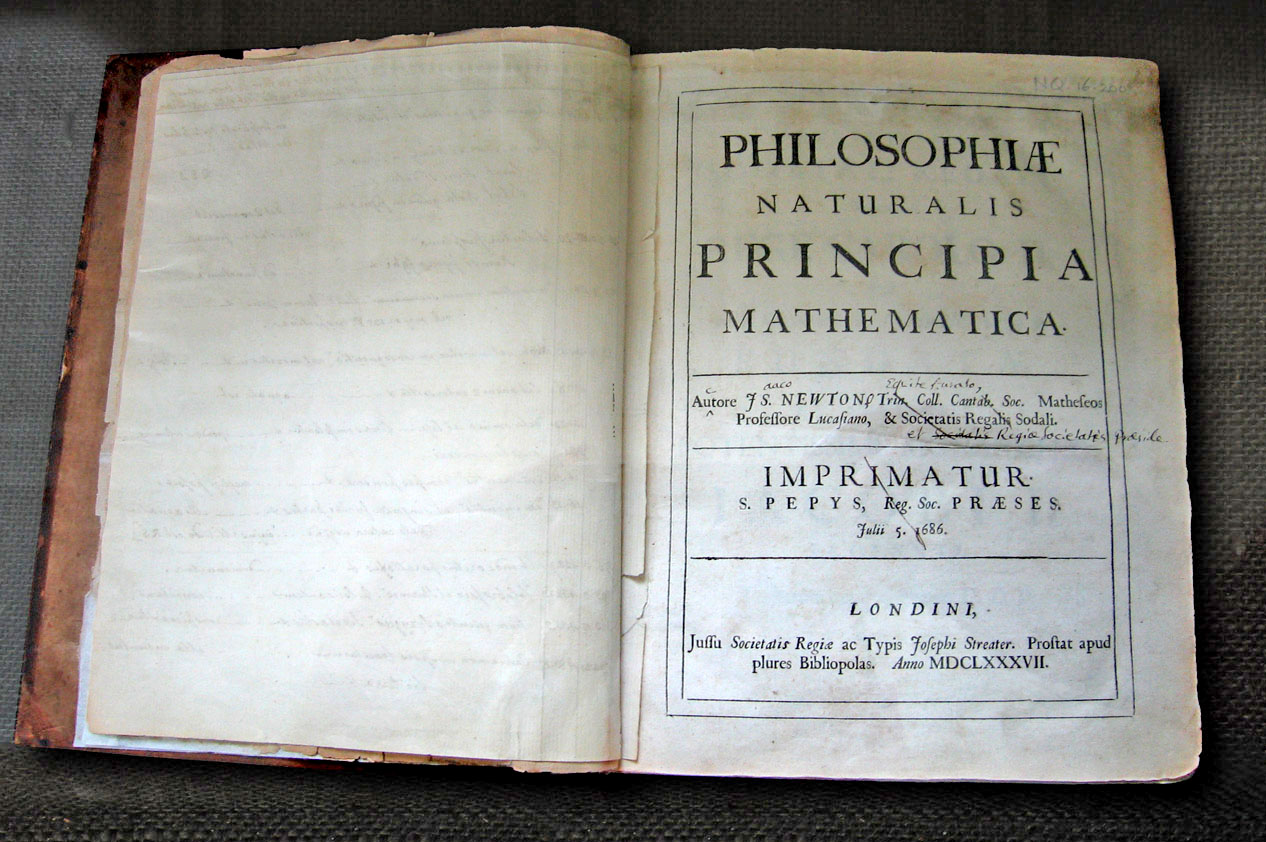
Fig. 7 Newton’s own copy of his Principia, with hand-written corrections for the second edition, in the Wren Library at Trinity College, Cambridge.

In this chapter we are going to look at some of the work that Isaac Newton developed way back in the 17^th century. Unfortunately we are not going to dabble in his obsession with alchemy1 or finding the Philosopher’s Stone, but instead will concern ourselves with a particular section of the “Philosophiæ Naturalis Principia Mathematica’’ published in 1687. In this work Newton defines three laws of motion that set the foundation for the field of classical mechanics which you will study in more depth next year.

You will already have seen these three laws of motion but there are some concepts or details that are often overlooked in pre-University courses so firstly we will review the three laws in turn before applying them to some representative examples.

I will forewarn you now that I’m going to make a point of including the original Latin of the three laws. There is some educational benefit to this, I assure you, but it is also a historical thing that makes students audibly groan during lectures in response to my “quirkiness”. I fully intend to honour this tradition until I retire.

First Law

Corpus omne perseverare in statu suo quiescendi vel movendi uniformiter in directum, nisi quatenus a viribus impressis cogitur statum illum mutare.

Every body persists in its state of being at rest or of moving uniformly straight forward, except insofar as it is compelled to change its state by force impressed.

The key point that I want to emphasise with this law is a subtle one but thinking about it now will help in the future when you start thinking about special relativity. Newton makes reference to the ‘state’ of the body. This state could be at rest or a constant motion straight forward but in all cases they are simply specifics of this general ‘state’. This state is the velocity of the body which means we can rephrase the First Law as

A body acted on by no net force moves with constant velocity.

The zero velocity case is simply a unique value in an almost infinite number of possible velocities. Sometimes it is convenient to make use of the zero velocity case, particularly when you start thinking about different frames of reference.

Second Law

Mutationem motus proportionalem esse vi motrici impressae, et fieri secundum lineam rectam qua vis illa imprimitur.

The alteration of motion is ever proportional to the motive force impress’d; and is made in the direction of the right line in which that force is impress’d.

This is by far the Law that is most frequently stated incorrectly. Or perhaps more accurately it is that the law taught to you in schools in a special case of a simplified version of the actual statement the Newton made. You will have heard people saying that the second law is simply \(F=ma\) however let us look at the original statement to see what information is missing when we look between the original and this simple-yet-incomplete definition.

What I hope you notice is that the original statement contains two key parts, conveniently separated by a semi colon. In the first part we have that the alteration of motion, or acceleration, is proportional to the applied force. This is all good and gels with our simple statement that \(F\propto a\), where the mass \(m\) is our constant of proportionality.

The information in the original definition that is lacking in our \(F=ma\) statement is that regarding the directions of the applied forces and the resulting acceleration.

Note

In this course I will be using the notation that a vector is denoted by bold font without italics.

When we want to combine information about the magnitude and direction of properties you should always think about vectors.

By combining the two components of the original statement for the Second Law we can give a more general statement of the law in mathematical form, namely that

(20)\[\textbf{F}=m\textbf{a}\]

Have you spotted the ‘error’ yet?

I was being rather picky with my choice of words right after the Latin and translation text. I said that the version taught is schools is both simplified and a special case. We have taken care of the simplification by including the directions by way of vectors but the special case element needs to be addressed.

Let us look back at equation (20). I was quite correct to not change the mass into a vector, but what I have assumed is that the mass is constant. In fact I need to go back to the original statement of the Second Law and think more generally about the “alteration of motion” and consider a property that contains both the velocity and mass of the body. This is, of course, the momentum \((\textbf{p}=m\textbf{v})\) of the body.

If we now reformulate the Second Law using this concept of the momentum into an equation we find that

(21)\[\textbf{F} = \frac{\mathrm{d}\textbf{p}}{\mathrm{d}t}\]

We can now check that this more general expression does reduce to the more familar form in equation (20) under special circumstances. Let us take equation (21) and apply the product rule

\[\begin{align*} \textbf{F} &= \frac{\mathrm{d}(m\textbf{v})}{\mathrm{d}t}=m\frac{\mathrm{d}\textbf{v}}{\mathrm{d}t} + \textbf{v}\frac{\mathrm{d}m}{\mathrm{d}t} \end{align*}\]

Because the rate of change of mass is zero

so in the special case that the mass remains constant the right hand term become zero and therefore we find that

\[\begin{align*} \textbf{F} &= m\frac{\mathrm{d}\textbf{v}}{\mathrm{d}t}\\ &= m\textbf{a} \end{align*}\]

but only when the mass is constant. You should try to rememorise Newton’s Second Law as the force applied to a body in a given time, also known as the impulse equals the rate of change of momentum of that body.

Third Law

Actioni contrariam semper et aequalem esse reactionem: sive corporum duorum actiones in se mutuo semper esse aequales et in partes contrarias dirigi.

To every action there is always an equal and opposite reaction: or the forces of two bodies on each other are always equal and are directed in opposite directions.

I won’t spend as much time on this Law as there is not as much to critique, but again the key point to emphasise is that in the original statement is there is mention of the magnitude and the direction of the forces. We can neaten this up slightly by introducing our good friends the vectors. If we consider a body A that is exerting a force of magnitude \(F_{AB}\) onto body B then body B exerts a force of magnitude \(F_{BA}\) onto body A, and so we can state that

\[\textbf{F}_{AB} = -\textbf{F}_{BA}\]

Summary of the three laws

Key point

1. First Law: A body acted on by no net force moves with constant velocity (which may be zero).

2. Second Law: The general mathematical form is \(\textbf{F}=\dfrac{\mathrm{d}\textbf{p}}{\mathrm{d}t}\). This reduces to \(\textbf{F}=m\textbf{a}\) only in the case where the mass remains constant.

3. Third Law: If body A exerts a force on body B, then body B exerts a force on body A of the same magnitude but in the opposite direction, i.e. \(\textbf{F}_{AB} = -\textbf{F}_{BA}\)

Resolving forces

The three Laws were discussed in quite some length but what we are really excited about is using these to solve some physics problems. So that is exactly what we will do now.

Example - Traffic Lights (not UK ones)

In this case we consider the type of traffic lights that are suspended from cables, as shows in Fig. 8 below. We have a traffic light suspended from a single cable which in turn is suspended from two cables that make angles of \(37.0^\circ\) and \(53.0^\circ\) to the horizontal beam above. We also know that the weight of the traffic light is \(125.0\text{ N}\), and we have been tasked with calculating the tensions in each of the three cables.

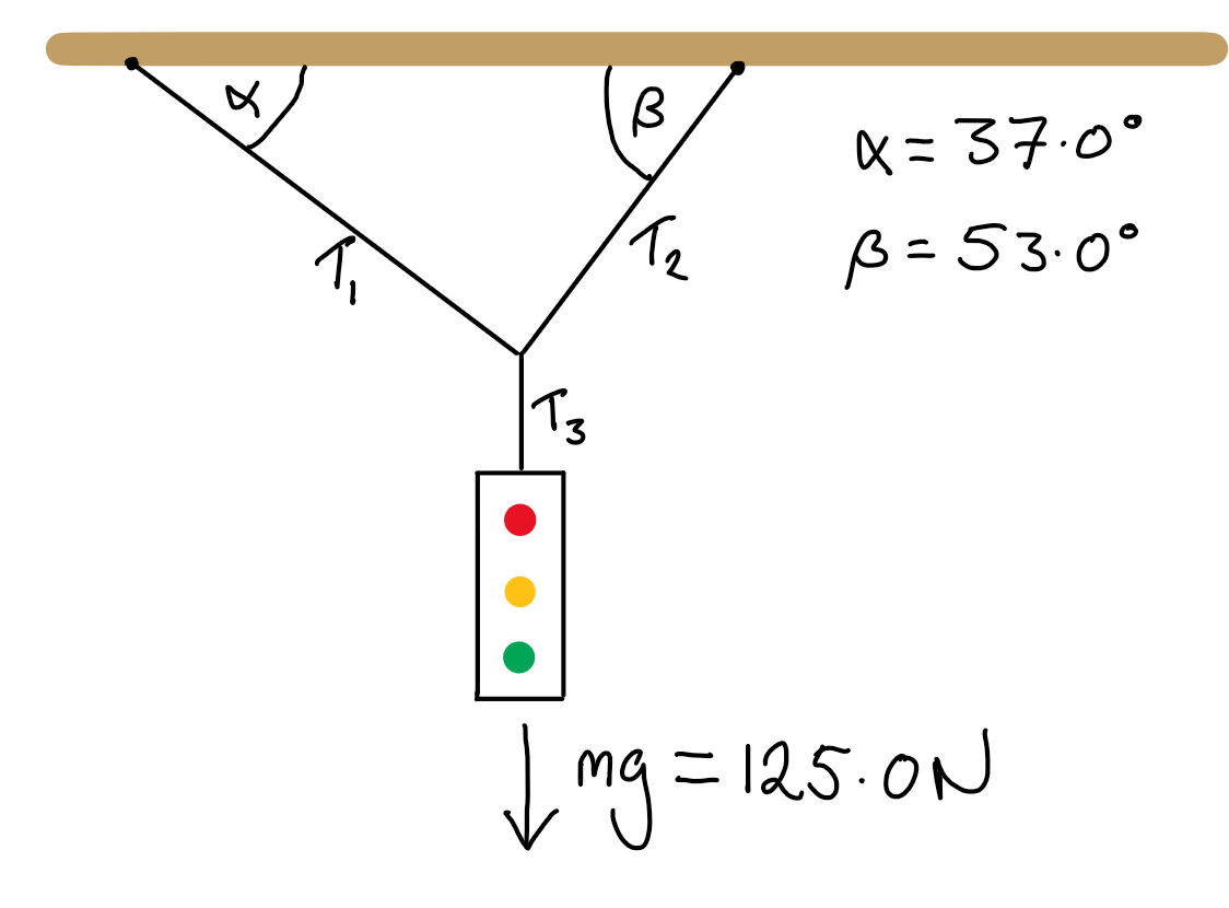
Fig. 8 A hanging style set of traffic lights suspended on one vertical wire which in turn is attached to two wires that are affixed to a horizontal surface. These two wires each make a different angle to this surface and so have a different tension. The traffic light is stationary so no velocity vectors are indicated.

Now before you jump straight in to the calculations we should take a step back and think a) about the assumptions of a system, and b) which approach we should take. The former is somewhat trivial but always worth stating: in this example I am assuming that the traffic light is stationary and therefore (from Newton’s First Law) there is zero net force in the system.

The latter point is important because taking a brief moment to pause and think about the approach gives you the time to think about which methods are valid and, of those, which are the most efficient. For the purposes of hammering this point home I’m going to solve this traffic light problem using two methods, the first being the typical approach taught in pre-University education and the second making use of the vectors that we emphasised in our earlier review of the three laws of motion.

Method 1 - Resolving components

Looking at Fig. 8 I am going to split the system up into two parts, the upper and lower, and will consider the lower part first. In this part I have two components, the weight of the traffic light \(mg\) and the tension \(T_3\). Both of these are only acting in the vertical direction which means

\[T_3 = mg\]

Note

As an aside, horizontal and vertical are somewhat arbitrary. What I am doing is splitting these into two orthogonal components, but given that gravity acts vertically it is sensible to align one of my components with this.

Next I consider the upper part and here I need to split the components of the three tensions into their horizontal and vertical components. Thus my horizontal components give

(22)\[\begin{split}T_1\cos\alpha &= T_2\cos\beta\nonumber\\ T_1 &= T_2\left(\frac{\cos\beta}{\cos\alpha}\right)\end{split}\]

Next our vertical components give

\[\begin{align*} T_3 = mg &= T_1\sin\alpha + T_2\sin\beta\\ &= T_2\left(\tan\alpha\cos\beta + \sin\beta\right)\\ \therefore T_2 &= \frac{mg}{\tan\alpha\cos\beta + \sin\beta} \approx 99.8\text{ N} \end{align*}\]

where I have substituted the expression for \(T_1\) (equation (22)) into the second line. Now that I have an expression or value for \(T_2\) I can substitute this back in to equation (22) to find

\[\begin{align*} T_1 &= T_2\left(\frac{\cos\beta}{\cos\alpha}\right)\\ &= \left(\frac{mg}{\tan\alpha\cos\beta + \sin\beta}\right)\left(\frac{\cos\beta}{\cos\alpha}\right) \\ &\approx 75.2\text{ N} \end{align*}\]

This precision is dictated by the precision of the original input values, in this case the weight and the two stated angles.

And there we have it. We have found that \(T_1=75.2\text{ N}\), \(T_2=99.8\text{ N}\) and \(T_3=125.0\text{ N}\) to the correct number of significant figures.

Method 2 - Vectors

The method above does work but it involved an unneccesary amount of work. By remembering that we are working with vectors we can avoid splitting our forces into their components of direction and magnitude (or in this case their horizontal and vertical), and just work with the vectors themselves.

We have assumed that the system is not accelerating which means there is no net force. Under this assumption the sum of the forces in the system should equal zero which, when expressed as a diagram, means the three vectors form a closed triangle when placed end to end. We will start by sketching this as in Fig. 9.

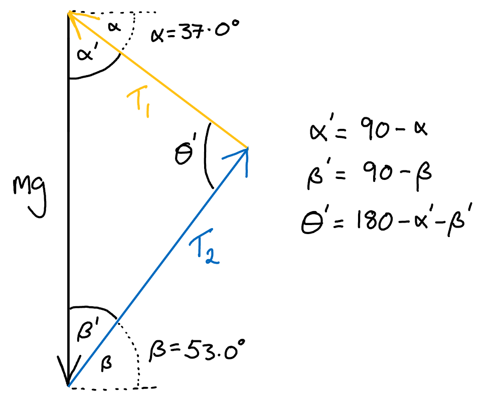
Fig. 9 Three arrows indicate the vector forces, one due to gravity pointing directly down, and the two force vectors point at angles with respect to the horizontal. The three vector arrows form a closed triangle because the traffic light is stationary and thus there is zero net force.

When presented in this form I hope it is fairly clear that we have a triangle with all lengths and angles defined (even if we do not yet know all the values).

Note

I’m borrowing the result from the previous method that \(T_3=mg\), but this is pretty obvious when you think about the system.

The fact that this is a triangle of vectors makes no difference; we can apply the geometry rules we all know and love to solve for the unknowns, in this case \(T_1\) and \(T_2\).

I will make use of the sine rules of triangles, which if you cannot remember it off the bat is defined as

\[\frac{mg}{\sin\theta'}=\frac{T_1}{\sin\beta'}=\frac{T_2}{\sin\alpha'}.\]

We know all of the parameters in the left hand side so will use this part twice, first to find \(T_1\) and again to find \(T_2\). For \(T_1\) this gives

\[\begin{align*} \frac{mg}{\sin\theta'}&=\frac{T_1}{\sin\beta'}\\ T_1&=mg\left(\frac{\sin\theta'}{\sin\beta'}\right)\\ &\approx0.602mg = 75.2\text{ N} \end{align*}\]

Similar steps will give you \(T_2 = 99.8\text{ N}\). These are the same as we found using the previous method, as we would expect, but the vector method is much more efficient

Mass on a string

This may all seem a little arbitrary and trivial but we can use the principles that allowed to solve the traffic light problem above to consider a different system that will form the basis of how you describe and manipulate waves on a string. All I will cover in this part of the course is from defining the system up to the definition of boundary conditions, but you will take this further in the Waves and Oscillations part of the module.

Our first step is one of defining some notation. Consider a string whose equilibrium position lies along the \(x\)-axis. If the string oscillates in the \(y\) direction only (that is, we confine this to two dimensions)

Note

\(\Psi\) is the Greek capital letter ‘psi’. You may ask why I’m not using \(A\) for amplitude, but typically \(A\) is the maximum amplitude whereas \(\Psi\) varies with time and position.

then the amplitude of the oscillation \(\Psi\) is a function of the position along the string and the time, denoted by \(\Psi(x,t)\) as shown in Fig. 10.

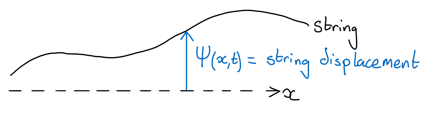
Fig. 10 The amplitude of each point on the string is a function of both the position along the string \(x\) and of time \(t\). This amplitude \(\Psi(x,t)\) is defined with respect to the equilibrium position, i.e. where the string sits stationary when no initial force or displacement is applied.

Let us consider a more complicated system of two strings that are joined together with a blob of glue with mass \(m\). These two strings have different mass densities, \(\mu_1\) and \(\mu_2\) but are both under the same tension \(T\). This can be seen in Fig. 11.

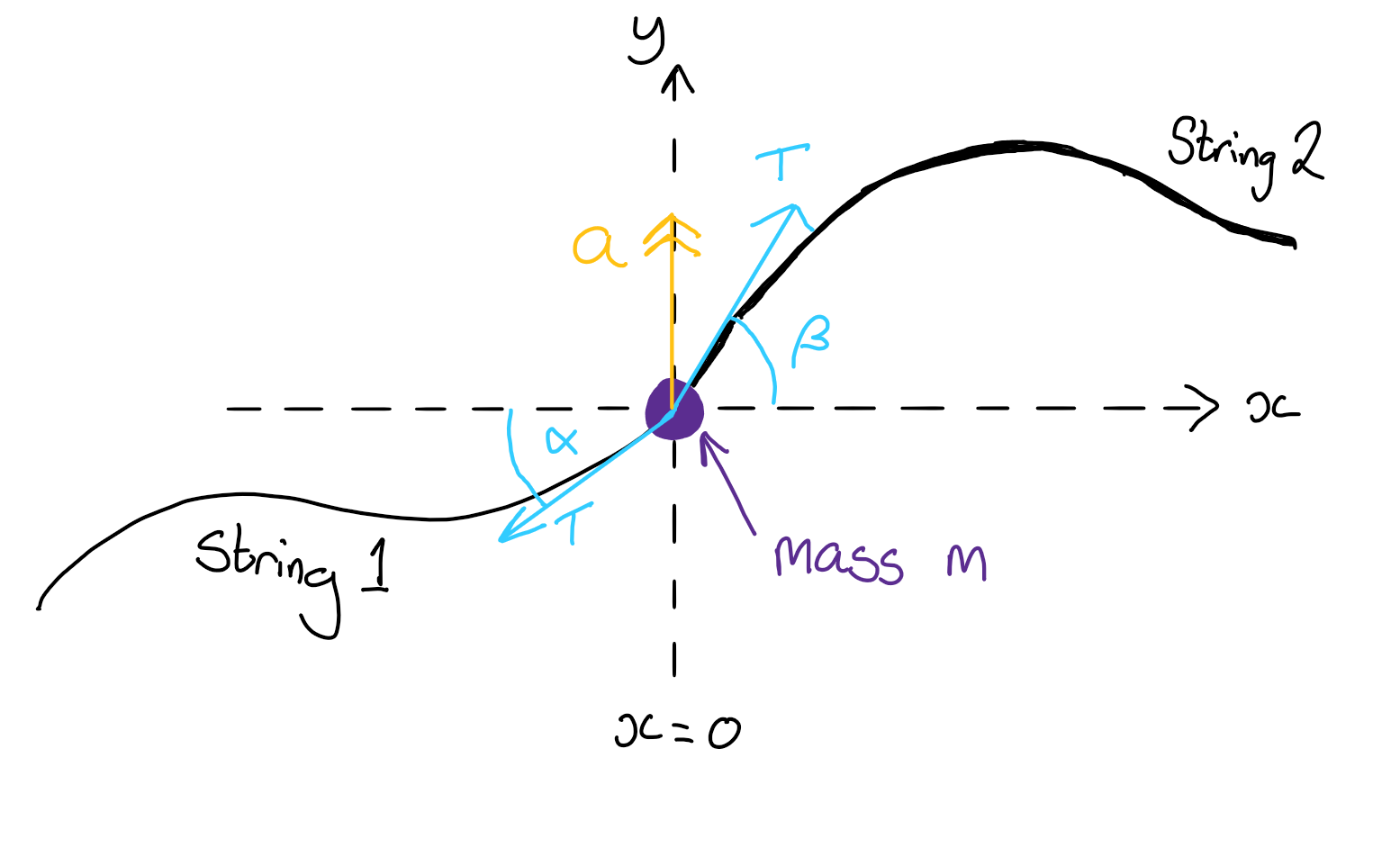
Fig. 11 A blob of glue with mass \(m\) is joining two strings of different mass densities together. As a wave travels along this string system the mass accelerates in the \(y\) direction only. There are two tensions acting on the mass, one from each of the strings.

Now we can start thinking about and defining the boundary conditions at the blob of glue which is the boundary between the two strings.

The first condition is that the strings must remain joined. This may seem silly and trivial but to ensure this condition is met at the boundary we can make some very useful statements. In order for the strings to remain joined any wave they are both carrying must have the same frequency at all points on the string and must have the same amplitude at the boundary . The string ends at the boundary cannot have different vertical positions if they are joined. Therefore at the boundary we can state

\[\begin{align*} \omega_1 &= \omega_2\\ \Psi_1(x=0,t) &= \Psi_2(x=0,t) \end{align*}\]

Note

In case you forgot, this is a lecture on forces!

The second boundary condition is less obvious from first glance but can easily be determined when we think about the forces acting on the blob of glue. The blob has an acceleration \(a\) which means

(23)\[T\sin\beta-T\sin\alpha =ma\]

For small oscillations we can state that

\[\begin{align*} \sin\beta \approx \tan\beta = \frac{\partial{\Psi_2}}{\partial{x}}(x=0,t)\\ \sin\alpha \approx \tan\alpha = \frac{\partial{\Psi_1}}{\partial{x}}(x=0,t) \end{align*}\]

We can also define the acceleration of the blob of glue in terms of the second partial derivative of the position with respect to time, i.e.

\[\begin{align*} a &= \frac{\partial{}^2\Psi}{\partial{t^2}} \end{align*}\]

We can substitute these three expressions back in to equation (23) to find

\[\begin{align*} T\frac{\partial{\Psi_2}}{\partial{x}}(x=0,t) -T\frac{\partial{\Psi_1}}{\partial{x}}(x=0,t) &= m\frac{\partial{}^2\Psi}{\partial{t^2}} \end{align*}\]

Finally let us suppose that there is no blob of glue at the join, such that \(m\rightarrow 0\), which leads to

\[\begin{align*} T\frac{\partial{\Psi_2}}{\partial{x}}(x=0,t) &= T\frac{\partial{\Psi_1}}{\partial{x}}(x=0,t)\\ \frac{\partial{\Psi_2}}{\partial{x}}(x=0,t) &= \frac{\partial{\Psi_1}}{\partial{x}}(x=0,t) \end{align*}\]

This can be reinterpreted as the curvature at the boundary is the same for both string 1 and 2. Intuitively this makes sense as we would not expect to see a sharp change in gradient at the boundary, and instead expect (or indeed require) it to be smooth.

So we now have our three boundary conditions:

1. \(\omega_1 = \omega_2\)

2. At \(x=0\), \(\Psi_1 = \Psi_2\) for all \(t\)

3. At \(x=0\), \(\dfrac{\partial{\Psi_1}}{\partial{x}} = \dfrac{\partial{\Psi_2}}{\partial{x}}\) for all \(t\)

These boundary conditions will allow you to solve for how waves scatter at the boundary between two strings which you will cover in the Waves and Oscillation lectures. Hopefully what you can see here is that these boundary conditions are fairly sensible to define when you think carefully about the physical system you are dealing with, and that even the more complicated one here about the requirement of continuous curvature at the boundary can be easily derived from some relatively simple resolution of forces.

Lecture Questions

Question 1

Question

Three vector forces \(\textbf{F}_1\), \(\textbf{F}_2\) and \(\textbf{F}_3\) act on a particle of mass \(m = 3.8\text{ kg}\) as shown below.

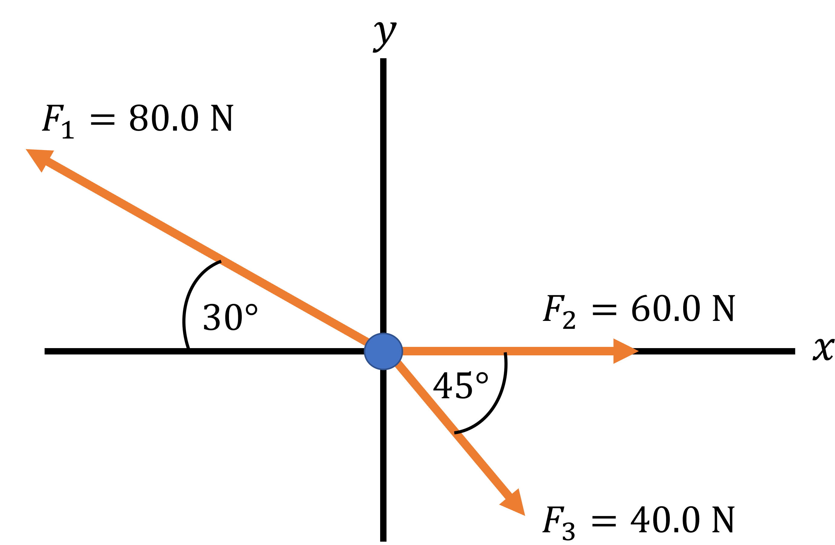
1. Calculate the magnitude and direction of the net force acting on the particle.

2. Calculate the particle’s acceleration.

3. If an additional stabilizing force \(\textbf{F}_4\) is applied to create an equilibrium condition with a resultant net force of zero, what would be the magnitude and direction of \(\textbf{F}_4\)?

Hint

Be careful with using the resolving vectors method. Not all of the vectors are labelled on the diagram, so you aren’t dealing with a triangle of arrows. However you could combine pairs of vectors into single vectors until you get down to three, and then use the triangle method.

Note that the word acceleration has a specific definition. Make sure you include all of the necessary information in your result.

Solution

1 The second step is to resolve the forces into \(x\) and \(y\) components. The first step is to check that it’s worth doing this! The question is asking for magnitude and directions, and the force diagram gives the three forces in magnitude and direction format, so it is indeed worth doing this.

\[\begin{align*} F_x &= -80\cos35^\circ + 60 + 40\cos45^\circ = 22.75\text{ N}\\ F_y &= 80\sin35^\circ + 0 - 40\sin45^\circ = 17.60\text{ N} \end{align*}\]

We can now calculate the magnitude of the net force \(F_\text{net}\) and the direction \(\theta\):

\[\begin{align*} F_\text{net} &= \sqrt{F_x^2+F_y^2}=28.8\text{ N}\\ \tan\theta &= \frac{F_y}{F_x} = 0.7736 \implies \theta = 37.7^\circ \end{align*}\]

where \(\theta\) is defined as anticlockwise from the positive \(x\) axis.

2

\[\begin{align*} a &= \frac{F_\text{net}}{m} = 7.6\text{ m s}^{-2} \end{align*}\]

in the direction of the force found in part 1 (i.e. \(37.7^\circ\) anticlockwise from the positive \(x\) axis).

3 The long approach to this question would be to go back to the first step but add another component into our expressions for \(F_x\) and \(F_y\) and then solving the simultaneous equations.

The shorter approach is to recognise that to have a net zero force one must add an additional force that is equal in magnitude but opposite in direction to \(\textbf{F}_\text{net}\), i.e. \(\textbf{F}_4 = -\textbf{F}_\text{net}\).

Question 2

Question

A container of mass \(200.0 \text{ kg}\) rests on the back of an open truck. If the truck accelerates at \(1.5 \text{ m s}^{-2}\), what is the minimum coefficient of static friction between the container and the bed of the truck required to prevent the container from sliding off the back of the truck?

Hint

A reminder that friction force is proportional to the weight of the object and acts parallel to the surface.

Solution

The force applied to the container \(F=ma\) and the frictional force \(F_f=\mu mg\). Therefore

\[\begin{align*} \mu mg &= ma\\ \therefore \mu &= \frac{a}{g} = 0.15 \end{align*}\]

Question 3

Question

Three strings are knotted together, and masses of \(7.0\text{ kg}\), \(8.0\text{ kg}\) and \(9.0\text{ kg}\) are attached to their free ends. The strings carrying the two lighter weights are slung over fixed smooth pegs. At what angle to the vertical do these strings rest when the system is in equillibrium?

Hint

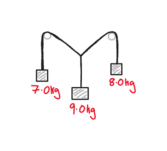
The pulleys are a slight distraction. How would the system change if you were to instead pull the \(7.0\text{ kg}\) and \(8.0\text{ kg}\) masses by the same force but in the direction of the diagonal lines connecting the \(9.0\text{ kg}\) mass cable and the two respective pulleys?

Solution

At equilibrium there is no net force. In terms of the force vectors this means the three involved should form a closed triangle from which we can use the cosine formula to calcuate our angles.

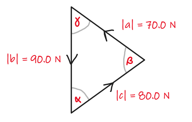
First we want to calculate \(\alpha\). We use

\[\begin{align*} a^2 &= b^2 + c^2 - 2bc\cos\alpha\\ \cos \alpha &= \frac{b^2 + c^2 - a^2}{2bc} = \frac{9600}{14400} = \frac{2}{3}\\ \therefore \alpha &\approx 42.1^\circ \approx 0.84\text{ radians} \end{align*}\]

The second angle we want to find is \(\gamma\) which is more obvious when you project upwards from the vectors \(a\) and \(b\). One again we use the cosine rule:

\[\begin{align*} c^2 &= a^2 + b^2 - 2bc\cos\alpha\\ \cos \gamma &= \frac{a^2 + b^2 - c^2}{2ab} = \frac{6600}{12600} \approx 0.52\\ \therefore \gamma &\approx 58.7^\circ \approx 1.02\text{ radians} \end{align*}\]

Strictly speaking there is a third angle that is needed, as the question asks for the angles that the three strings make to the vertical. The third string i.e. vector \(\textbf{b}\) is pointing vertically down so the angle is either zero or \(\pi\) radians depending on which way you define the positive vertical axis.

Question 4

Question

An aircraft of mass 10 metric tonnes is gliding at \(5^\circ\) to the horizontal. The pilot has turned the engine meaning that the plane is gliding at a constant speed. Determine the forces of lift and drag.

Note: 1 metric tonne is \(10^3\text{ kg}.\)

Hint

Avoid the temptation to assume that lift acts vertically with respect to the ground, and that drag acts horizontally. These two forces act on the aircraft, so think in terms of how the aircraft moves.

Solution

The weight of the aircraft is \(10^3g\) - I’m leaving it in terms of \(g\) for now and will plug numbers in at the end.

The lift force \(L\) is the force which keeps an aircraft in the air and acts perpendicular to the direction of motion. On the other hand the drag force \(D\) acts anti-parallel to (i.e. parallel to but in the opposite direction of) the direction of motion.

As the speed of the aircraft is constant the forces must be in equilibrium. We can therefore construct a force triangle from which we can determine

\[\begin{align*} D &= 10^3g\times\sin5 = 855.0\text{ N}\\ L &= 10^3g\times\cos5 = 9772.7\text{ N} \end{align*}\]

---

1

Sorry to any Fullmetal Alchemist fans out there