
Lecture 8 - Rotational motion and moments of inertia#
In Lecture 7 we considered the forces acting on a circular system. What you will find, if you haven’t spotted it already, is that there is generally a rotational counterpart to all of the linear topics we have studied so far. Last time we looked at forces and in this chapter we are going to consider the kinematic equations for a rotating system, before moving on to consider how we need to rethink mass for rotating objects.
Rotational motion for constant angular acceleration systems#
We are going to only consider rotating systems that have a constant angular acceleration \(\alpha_0\). If our angular acceleration is constant then
but we can also make use of the definition that the angular acceleration is the rate of change of angular velocity \(\omega\), thus
We can substitute in \(t=0\) to find this constant of integration because \(\omega(t=0)\) is simply the initial angular velocity \(\omega_0\), so \(c_1 = \omega_0\). Therefore
Take a moment to look at this expression. It looks remarkably similar to the constant acceleration kinematic equations for a linear system, in this case the \(v(t) = at + v_0\) equation. Swap linear velocities \(v\) for angular velocities \(\omega\), and do the same for accelerations \(a\) to \(\alpha\), and you can easily remember one set if you remember the other set.
For completeness though we will actually derive the kinematic equation for angular displacement. Starting from equation (50) and noting that the angular velocity is the rate of change of angle we can show
Once again we make use of the initial conditions that for when \(t=0\) we have the initial displacement \(\theta(t=0)=\theta_0\) so putting these into the equation above means that \(c_2 = \theta_0\). So finally we find
You should hopefully be able to see the similarites between this equation and the linear kinematic equation counterpart (\(x(t) = \frac{at^2}{2}+v_0t+x_0)\).
Using these kinematic equations is very similar to the linear version. You will get more practice of these in the tutorials and homeworks but you can find other practice questions in any undergraduate physics textbook.
Energy of a rotating body#
A logical next step will be to consider the total kinetic energy of a rotating body, firstly by examining an individual particle moving on a circular path but then developing this idea to an extended solid body rotating about some axis.
For the individual particle case we use our standard equation for the kinetic energy but note that the velocity is the tangential velocity. A justification for this is that if the centripetal force were to suddenly vanish the particle would move off in a straight line at the tengential velocity and therefore would have kinetic energy \(\frac{1}{1}mv_t^2\). However we now have an relationship between the tangential and angular velocities which allows us to define the kinetic energy of an individual particle moving in a circular path of radius \(r_i\) as
where the subscripts \(i\) indicate an individual particle, notation that will become very useful shortly.
Let us now move on to the extended solid body case. The way we treat this system is by breaking the single solid body down into the sum of individual particles all rotating about a common axis. It then follows that the total kinetic energy of the solid body is equal to the sum of the kinetic energies of these individual particles.
In Fig. 22 I have picked out two specific particles, labelled with subscripts 1 and 2, to highlight the differences. Particle 1 of mass \(m_1\) follows a circular path of radius \(r_1\) and has tangential velocity \(v_1\) whereas particle two has different mass \(m_2\), radius \(r_2\) and tangential velocity \(v_2\). What they do have in common is the angular velocity \(\omega\) - the angular velocity must be the same for all particles that make up the solid body if the body were to remain in the same shape and not skew or distort. You’ll also note that I have not made the assumption here that the masses of each particle are the same. This allows me to be more general in the subsequent treatments for bodies that have non-uniform densities, although in practice we will usually stick to the uniform case when solving problems in this course.
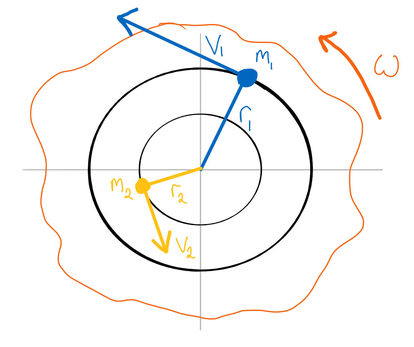
Fig. 22 A randomly shaped blob rotating about some axis. This mass is split into small pieces, each of which have their own distance from the axis of rotation and tangential velocity. All mass pieces are moving with the same angular velocity.#
The total kinetic energy \(KE_T\) of the solid body is the sum of the individual kinetic energies of the particles, and so
where \(I\) is the moment of inertia defined by \(\sum_im_ir_i^2\). Note that this equation for the total kinetic energy is similar to the equation for our linear systems \(\left(\frac{mv^2}{2}\right)\) where \(\omega\) is the rotational counterpart to \(v\) and \(I\) is therefore the counterpart to \(m\). But what exactly is the moment of inertia? Why does the “mass like” term in the kinetic energy of a rotating body have units of mass \(\times\) length\(^2\)?
Moment of inertia#
Note
This topic is historically the one that students find the most difficult of the entire Mechanics course. So if you do not understand it immediately, don’t worry. It is something that makes more sense when you re-read it a few times in conjunction with working through some derivations and practice questions.
To get an understanding of what moment of inertia is I want to return to our old friend Newton’s Second Law but to reframe what it means. Taking the simple case where the mass remains constant, i.e. we use \(F=ma\) then it is possible to redefine the mass as a measure of resistance to changes in linear motion. In the Second Law equation \(m\) is a constant of proportionality and if this constant is larger then a larger force is required to cause the same acceleration (hence being a measure of resistance).
The moment of inertia is the rotational analogue; it is the resistance to changes in rotational motion.
There is a key difference between mass and moment of inertia. The mass of an object is intrinsic to it, and when we want to accelerate a body of mass \(m\) along a straight line it does not matter how this mass is distributed. The same is not true for a rotating body. The resistance to changing the rotational motion of a body depends not only on how much mass the body has but how this mass is distributed with respect to the axis of rotation. We will explore this further in a couple of worked examples below and some in your tutorials, but table 9.2 in the core textbook shows the range of geometries we will consider in this course.
Before we embark on some worked examples we need to make one final adjustment to our definition of the moment of inertia. In the definition above we are taking a simple summation of discrete particles of equal mass \(\Delta m\) but it is more useful to take the limit of this as the masses tend to \(0\)
The general procedure for solving this integral is:
Split the body up into small mass elements \(\mathrm{d}m\)
Change \(\mathrm{d}m\) into a distance element, assuming the body has a uniform density.
Integrate equation (51) over this substituted distance element, noting that the limits should cover the whole length of the body with respect to the axis of rotation.
In some cases we can deviate from this general procedure but this is very much dependent on the geometry of the system.
Important
All moment of inertias will be of the form \(cMR^2\) or \(cML^2\), i.e mass times distance squared, with some numerical prefactor \(c\) that depends on the geometry of the system and the location of the axis of rotation.
Moment of inertia of a ring / thin cylinder
Consider a ring or hoop of mass \(M\) and radius \(R\) rotating in the \((x,y)\) plane with the origin at the centre of the ring (i.e. the centre of mass). We split the hoop up into an infinite number of thin slices each of mass \(\mathrm{d}m\), as shown in Fig. 23.
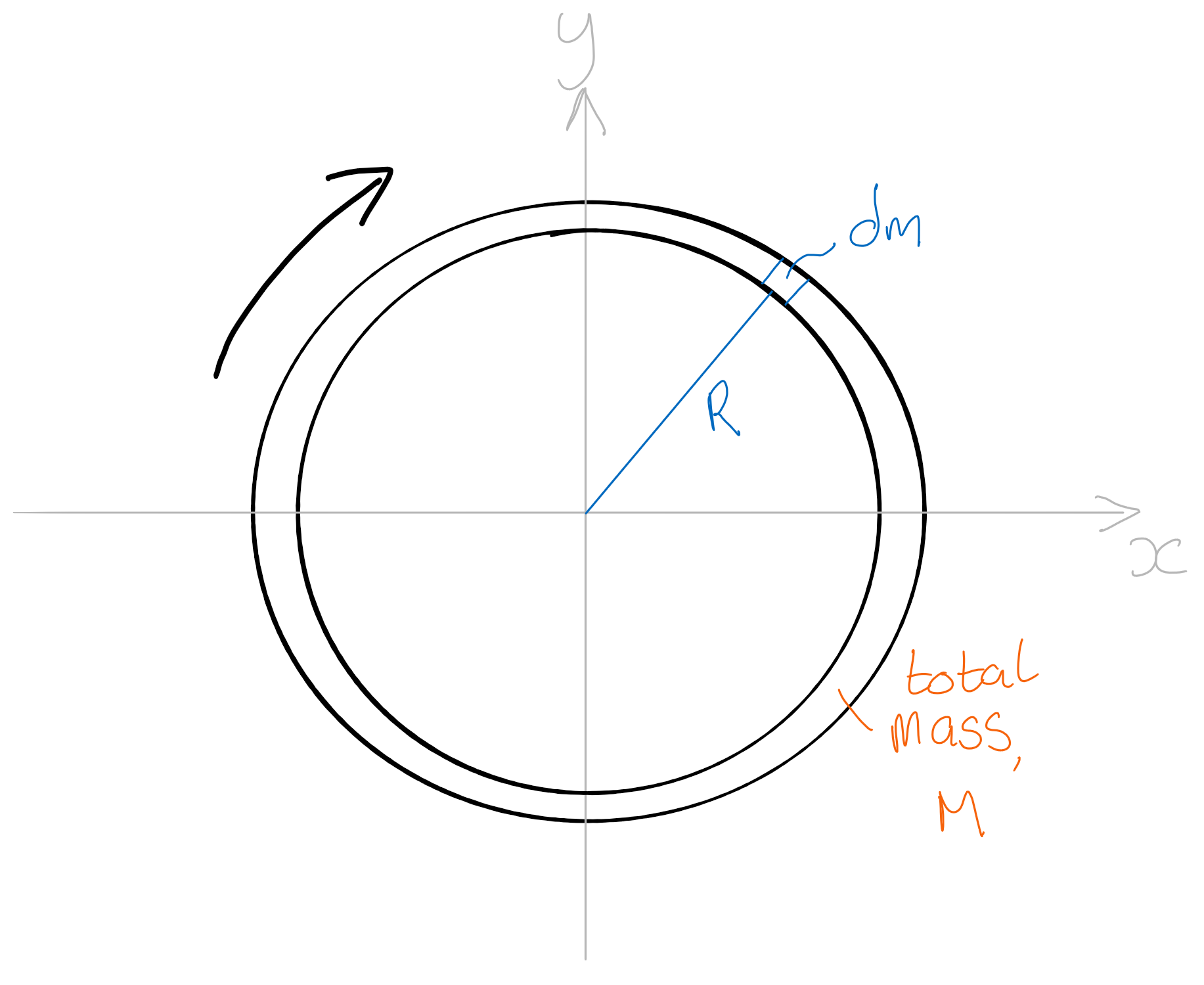
Fig. 23 A thin hoop of mass \(M\) rotating about a point through the centre of the hoop and perpendicular to the plane of the hoop. The hoop is split into small mass elements, each of which are a distance \(R\) from the axis of rotation.#
At this point we can deviate slightly from the general procedure I set out previously. The reason we can do this for a hoop or ring is because in this very specific geometry and axis configuration the distance of each of the elements to the axis is constant, in this case it is the radius of the hoop. This means that for this example we can take \(R\) outside of the integral which gives
Moment of inertia of a thin uniform rod
Consider a thin uniform rod of mass \(m\) and length \(L\) as shown in figure Fig. 24. By “thin” we assume the radius of the rod is negligible. We first rotate the rod about an axis perpendicular to the length of the rod and passing through the centre of mass (labelled (a) in the figure).
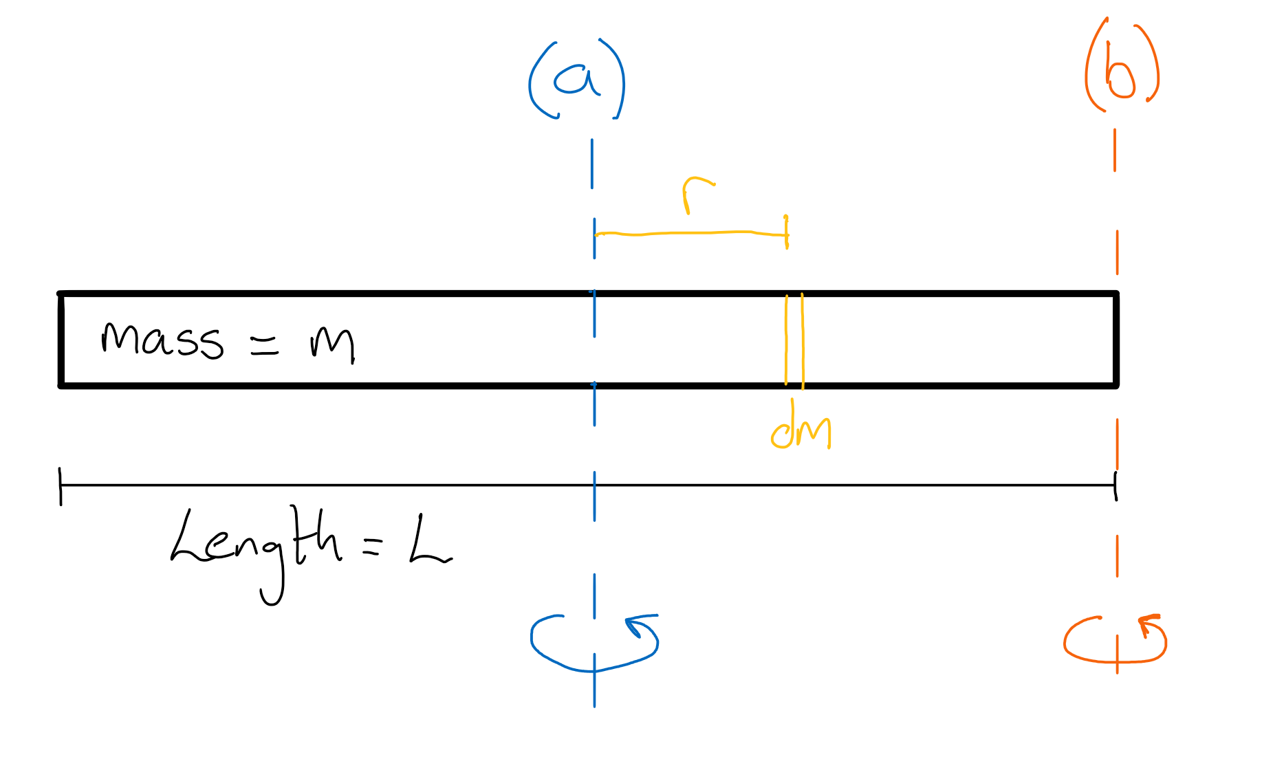
Fig. 24 Schematic of a thin uniform rod of mass \(m\) and length \(L\) rotating about an axis a) through the centre of the bar or b) through the end of the bar. Both axes are perpendicular to the length of the bar. The bar is split into small masses, each some distance \(r\) from the axis of rotation.#
We need to split our rod up into thin slices with mass elements \(\mathrm{d}m\) each with their own distance \(r\) from the axis of rotation. Now we cannot simply integrate the variable \(r\) with respect to \(\mathrm{d}m\) - we need to change one of these parameters into the same units as the other. To do this we make use of the fact that the rod is uniform which means the linear mass density \(\lambda\) of the whole rod is the same as the density for our thin mass element of thickness \(\mathrm{d}r\). Thus
We substitute this expression into our general form for the moment of inertial (equation (51)) and solve
Spinning a rod about the centre is not the only way to do it. What happens if instead we spin the exact same rod about one of the end points, in this case the axis labelled (b) in Fig. 24? The derivation above is identical however because our zero point is now at one end of the bar we need to change the limits of integration. Therefore
So we have two different moments of inertia for the exact same rod. The difference here is that the location of the axis of rotation changes, so you must be vigilant and explicit in defining your axes. A diagram will always help.
Moment of inertia of a thin hollow sphere (a shell)
There are a number of ways to calculate the moment of inertia of a shell rotating about an axis that passes through the centre of mass (i.e. through the diameter of the shell). In the core textbook they show how you can construct this moment of inertia as the sum of an infinite number of thin hoops who radii increase and decrease from top to bottom of the shell. This works but because this approach uses Cartesian coordinates to describe a spherical system the algebra can get a little messy. Instead I am going to describe an alternative approach that makes use of spherical coordinate systems which are, by their very definition, well suited for describing spherical systems.
Firstly we split the shell up into small rectangles of area \(\mathrm{d}A\). We use the spherical coordinates \(R\) as the distance from the origin to the volume element, \(\theta\) is the azimuthal angle and \(\phi\) is the zenith angle. These are shown in Fig. 25.
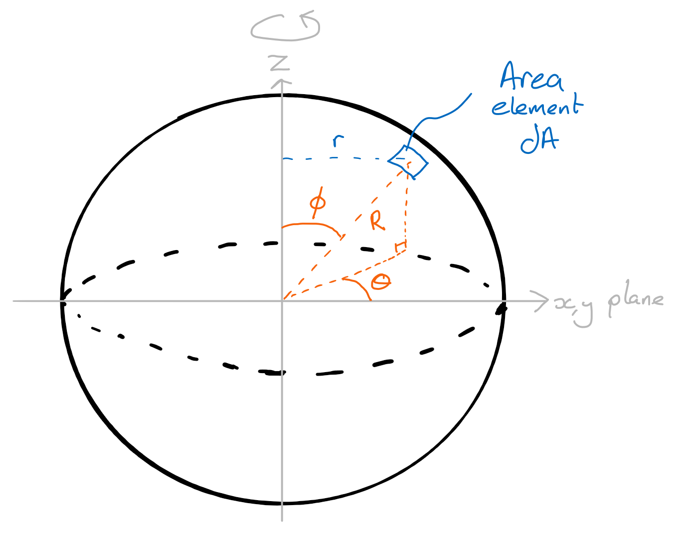
Fig. 25 Schematic of a thin spherical shell rotating about an axis through the diameter of the shell. The mass is split into small surface areas with the small area defined using spherical polar coordinates \((r,\theta,\phi)\).#
This area element can be defined in terms of the three components of the spherical coordinate system, namely
and so the mass of this area element is
where \(\sigma\) is the area density (mass per unit area). We next need to determine an expression for the distance from the axis of rotation to the mass element, which is not the same as \(R\). Some simple trigonometry tells us that \(r=R\sin\phi\), and we can now substitute this into our mass element expression above which in turn we substitute into equation (51) and solve:
To solve this integral we use a fairly common technique that you should see in your maths course but I will show without explanation here.
We can use this result for the integral in equation (52) to finally find
where we have used \(\sigma = \dfrac{M}{4\pi R^2}\) by definition.
Moment of inertia of solid sphere
This system shares a lot of similarities with the thin hollow sphere, but instead of adding up lots of small area elements \(\mathrm{d}A\) we instead need to add up lots of small volume elements \(\mathrm{d}V\).
We also can no longer set the radius as a constant value \(R\), as the small volume elements range from at the centre of the sphere out to the edge. If the define this distance to origin of the volume element as \(s\) then we can state \(0\leq s \leq R\).
Thus
where \(\rho\) is the density of the sphere.
Using the same definition for \(r\) as in the thin hollow shell case we now find that
which allows us to find
Finally we use \(\rho = \frac{M}{V}=\frac{3M}{4\pi R^3}\) to find
Using symmetry#
All of the examples we have considered so far have been solved by adding up the moment of inertia contributions from small point masses across the whole extended shape we are interested in. In other words
This may seem a silly statement to make but it does allow us to leverage symmetry to make the process easier for certain shapes. If it is possible to construct one shape out of an infinite number of another shape for which we know the moment of inertia expression, then we can use (53) with the moment of inertia for these “infinite shapes” on the right hand side.
This is a lot clearer by going through two more examples, the solid disc and the solid sphere.
Moment of inertia of a thin solid disc
We can consider a solid disc to be made up of a series of infinitely thin concentric rings of increasing radii, starting from \(r=0\) and going up to \(r=R\). We know the moment of inertia of a ring is \(I_\text{ring}= MR^2\) so an infinitesimal ring is
where the surface area of a hoop of infinitesimal thickness is \(\mathrm{d}A=2\pi r\,\mathrm{d}r\).
Substitute this expression into (53) gives
You can derive this from small mass elements, like we’ve done in the previous examples. That’s an exercise for you to try if you want - you will get the same result as above.
Moment of inertia of solid sphere - shell method
The conceptual idea here is that a solid sphere can be made from an infinite series of infinitely thin shells, a bit like an onion. So the total moment of inertia is
where
where the expression \(\mathrm{d}V=4\pi r^2 \mathrm{d}r\) is the volume of a thin shell of radius \(r\) and thickness \(\mathrm{d}r\). Thus
Before I finish, it’s worth pointing out that there is another way to derive the moment of inertia for a solid sphere. Instead of adding up an infinite number of thin shells you can add up an infinite number of discs, stacked on the \(z\) axis going from a very small radius (at \(z=R\)), up to a maximum of \(R\), then back down to very small at \(z=-R\). I’m not going to derive this here as it’s in the core textbook and a number of websites.
Axis theorems for moments of inertia#
In the real world we often want to calculate the moment of inertia for a body about an axis that does not lend itself to a nice symmetry of mass distribution. You will see this in one of the tutorial questions where we examine in great depth the opening of a swing bin lid.
There are two theorems that come to our aid, the parallel axis theorem and the perpendicular axis theorem. These are extremely useful as they allow us to translate from rotation about one axis to another axis so long as the new one is either parallel or perpendicular to the first axis. In practice this means we often start with one of the nice symmetric systems and shift our axes to suit.
For example if we wanted to calculate the moment of inertia of a hula hoop being spun around on your wrist then we can start with the moment of inertia for the hoop through the centre of mass (i.e. the centre of the hoop) and shift the axis by a distance equal to the radius of the hoop.
You are able to prove these theorems fairly easily but for the purpose of this course you will not be expected to remember the proofs. The results are worth remembering but knowing how to derive them can be helpful in a pinch if you cannot remember the final equations.
Paralled axis theorem#
The moment of inertia about a parallel axis some distance \(D\) away from the centre of mass axis is
Perpendicular axis theorem#
If the moments of inertia about the \(x\) and \(y\) axis are known then the moment of inertia about \(z\) is
Note that my choice of \(x\), \(y\) and \(z\) is arbitrary. \(I_x = I_y + I_z\) is equally valid. The important point is that the three axes involved are perpendicular to each other.
Lecture Questions#
Question 1
The cable supporting an elevator runs over a wheel of radius \(R=0.36\text{ m}\). If the elevator begins from rest and ascends with an upward acceleration of \(0.60\text{ m s}^{-1}\), what is the angular acceleration of the wheel? How many turns does the wheel make if this accelerated motion lasts \(5.0\text{ s}\)?
Assume that the cable runs over the wheel without slipping.
Think about what the “no slipping” condition means in terms of the velocity of the wheel and the cable.
Also note that the question asks for the number of turns.
If there is no slipping then the speed of the cable must always equal the tangential speed of a point on the rim of the wheel. The acceleration of the elevator must therefore be the same as the tangential acceleration of a point on the rim of the wheel, such that
The angular displacement over this 5.0 s period is
The question asks for the number of turns which is found from
Question 2
A motor rotates a circular saw wheel, beginning from rest, with an angular acceleration that has an initial value \(\alpha_0 = 60\text{ radians s}^{-2}\) at \(t=0\) and decreases to zero acceleration during the interval \(0\leq t\leq3.0\text{ s}\) according to
After \(t=3.0\text{ s}\) the motor maintains the wheel’s angular velocity at a constant value.
What is the final constant angular velocity?
How many revolutions occur in the process of the wheel “getting up to speed” (i.e. in the time between \(t=0\) and \(t=3\))?
Remember to check your assumptions before jumping straight into the memorised equations of motion. Constant acceleration isn’t always the case…
1 The angular acceleration is given as an explicit function of time so we cannot simply use the constant angular acceleration kinematic equations. But we know the form the acceleration takes (given in the question) so we can solve using \(\alpha = \frac{\mathrm{d}\omega}{\mathrm{d}t}\)
where we make use the initial condition that \(\omega_0=0\). Substituting the value for \(t=3\) gives \(\omega = 90\text{ radians s}^{-1}\).
2 We need to find the change in angular position over the stated time period, which is found using \( \omega= \dfrac{\mathrm{d}\phi}{\mathrm{d}t}\) and the expression for \(\omega(t)\) found in part (1).
Evaluating this at \(t=3.0\text{ s}\) gives \(\Delta\phi = 180\text{ radians}\) and so the number of revolutions \(=\dfrac{180}{2\pi} = 29\text{ revolutions}\).
Question 3
Two people are sitting on a massless seesaw, on either side of the fulcrum (i.e the pivot point). Person \(L\) is on the left of the fulcrum at a distance of \(1.85\) m and has mass \(50\) kg whereas person \(R\) on the right is \(1.15\) m from the fulcrum and has mass \(80\) kg. If the (instantaenous) angular velocity of the seesaw is \(0.40\text{ radians s}^{-1}\) and assuming the people are particles(!), calculate the kinetic energy of the system by considering:
the individual kinetic energies of the people / particles,
the single system comprised of both people / particles.
This is a mixture of linear kinematics and rotational kinematics. Be careful to use the right one in the right place.
1 Treating the people as individual particles means the kinetic energy is found from their corresponding tangential velocities, i.e.
So the kinetic energies are
and so the total kinetic energy \(K_T=K_L+K_R = 22\text{ J}\).
2 To consider the seesaw + people as a single system we need to find the moment of inertia for the whole setup. As the seesaw is of negligible mass we treat our system as two particles rotating about some common axis (in this case the pivot point of the seesaw).
The total moment of inertia for a series of points is the sum of the individual moments of inertia, meaning
The kinetic energy of rotational motion for this single system is thus
Note that we get the same answer from both parts of this question which is to be expected!
Question 4
Find the moment of inertia of a wide ring (or annulus), made from a uniform but thin sheet metal of inner radius \(R_1\), outer radius \(R_2\) and mass \(M\) rotating about its axis of symmetry.
As with all moment of inertia problems, what is the system of shapes that you can “build up” to give you the system you are trying to model? Remember that similar symmetry and a shared axis of rotation is important.
The annulus can be regarded as made of a large number of thin, concentric hoops fitting arround one another, each with radius \(R\) and (infinitesimal) width \(\mathrm{d}R\). All of the mass \(\mathrm{d}m\) of this hoop is the same radius \(R\) from the axis of rotation therefore the moment of inertia of a hoop is
The area \(\mathrm{d}A\) of the hoop is the circumference times the width, i.e.
The mass of the hoop is the surface density times the hoop area
where I have made use of the fact that the material is uniform and so the area density of the thin hoop is the same as the whole annulus, i.e.
Thus the moment of inertia is
It is worth noting that if \(R_1=0\) our system becomes a solid disc and gives the expected moment of inertia i.e. \(I_{\text{disc}}=\frac{MR^2}{2}\). Similarly if \(R_1=R_2\) our system becomes a single hoop and the above equation reduces to the form expected i.e. \(I_{\text{hoop}} = MR^2\).