1.2 Shearing a solid or liquid

1.2 Shearing a solid or liquid#

In the previous sections we have discussed the differences between hard and soft condensed matter in terms of a) the types of units (atoms versus long molecules) and b) the relative strength of inter-unit bonds. These are both valid distinctions (otherwise I wouldn’t be including them here) but from a historical and pragmatic perspective they are very difficult to observe. In practice a great deal of the developments in understanding soft condensed matter came from observing the macroscopic properties of materials and developing theories and predictions of molecular systems and interactions that could lead to the properties we measure in the everyday world.

Consequently we are now going to turn our attention to the differences between hard- and soft- condensed matter at the macroscopic or bulk level. But to do so we need to consider the simple cases we are already familiar with, namely a Hookean solid (i.e. one that obeys Hooke’s law) and a Newtonian liquid, and then we will consider materials that deviate away from one or both of these ideal materials.

Hookean solids and Newtonian liquids#

Shearing a solid - stress and strain#

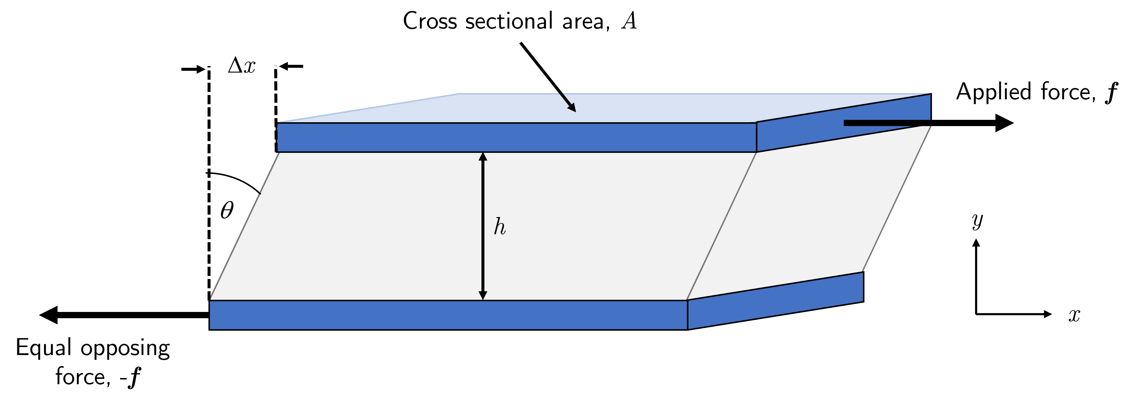
$Simple shear applied to a material (grey) fixed between two flat plates (blue) with surface area $A$. The bottom plate is fixed in place and a force $f$ is applied to the top plate along the $x$ direction that results in a deformation of the material by some distance $\Delta x$. \\Note that as the system is not moving there must be an equal and opposite force holding the bottom plate in place, rather than it being moved along with the force transmitted from the top plate through the material.$

Fig. 5 Simple shear applied to a material (grey) fixed between two flat plates (blue) with surface area $A$. The bottom plate is fixed in place and a force $f$ is applied to the top plate along the $x$ direction that results in a deformation of the material by some distance $\Delta x$. \Note that as the system is not moving there must be an equal and opposite force holding the bottom plate in place, rather than it being moved along with the force transmitted from the top plate through the material.#

Consider the system presented in Fig. 5 in which a solid material is fixed between two plates (of cross sectional area $A$). Firstly we assume that the bottom plate is fixed, and that the adhesion between the material and the plates is sufficient strong that there is not slippage between material and plate. A horizontal force $f$ is applied to the top plate which results in the top plate, and thus the top of the solid material being moved some distance $\Delta x$ from the equilibrium position. As the bottom plate is connected to the top via the material then any force that is applied to the top plate is ‘transmitted through’ to the bottom plate, but as the bottom plate is fixed there must be an equal and opposite force acting to keep it stationary.

The shear stress $\sigma$ is defined as the ratio of the force applied and the cross sectional area of the surfaces. This area is also the area of any plane in the material parallel to the plane of the plates, meaning that any horizontal slice through the material experiences the same shear stress. We can thus state that

(1)#\[\sigma = \frac{f}{A}\]

Next we turn our attention back to the observation that applying this force to the top plate causes it to displace by some distance $\Delta x$. The shear strain $\gamma$ is the ratio of this displacement and the thickness of the sample $h$, namely

(2)#\[\begin{split}\gamma &= \frac{\Delta x}{h}\\ &= \tan\theta \\ &\approx \theta \text{ for small displacements}\end{split}\]

We are making the assumption here that the separation between the plates, i.e. the thickness of the sample, remains constant. In reality at large displacements of the top plate we would expect the material to thin as it becomes more spread out, but we tend to measure samples under small displacements partly for this reason but also in part that hard solids tend not to move much!

If the material is a perfectly elastic solid then the shear strain (how much it moves for a given thickness) is proportional to the shear stress (how much force is applied to a cross sectional area). The constant of proportionality is called the shear modulus $G$ and is thus

(3)#\[\begin{split}G&= \frac{\sigma}{\gamma}\\ &\left(= \frac{f}{A}\frac{h}{\Delta x}\right)\end{split}\]

Tensile stress and Young’s modulus#

You might feel that the shear modulus has the same look as Young’s modulus, and indeed there are some parallels. It is important to differentiate between these two moduli as Young’s deals with axial (typically linear) stress-strain whereas the shear modulus considers a system undergoing shear. For completeness Young’s modulus is defined as

(4)#\[Y = \frac{\sigma_\text{tensile}}{\varepsilon} = \frac{f}{A}\frac{L}{\Delta L}\]

though I am making the assumption that this is a topic you have already covered previously and so only stating the final relationship.

Poisson’s ratio#

One of the assumptions made in both defining the shear and Young’s moduli is that applying the stress in one direction does not change the dimensions in other directions; the material being tested does not get thinner as it is sheared or stretched.
In reality we know that this is rarely the case. For the tensile (Young’s) case we can define Poisson’s ratio $\nu$ which considers how a longitudinal strain can result in a lateral or transverse strain. Consider the two dimensional case shown in Fig. 6.

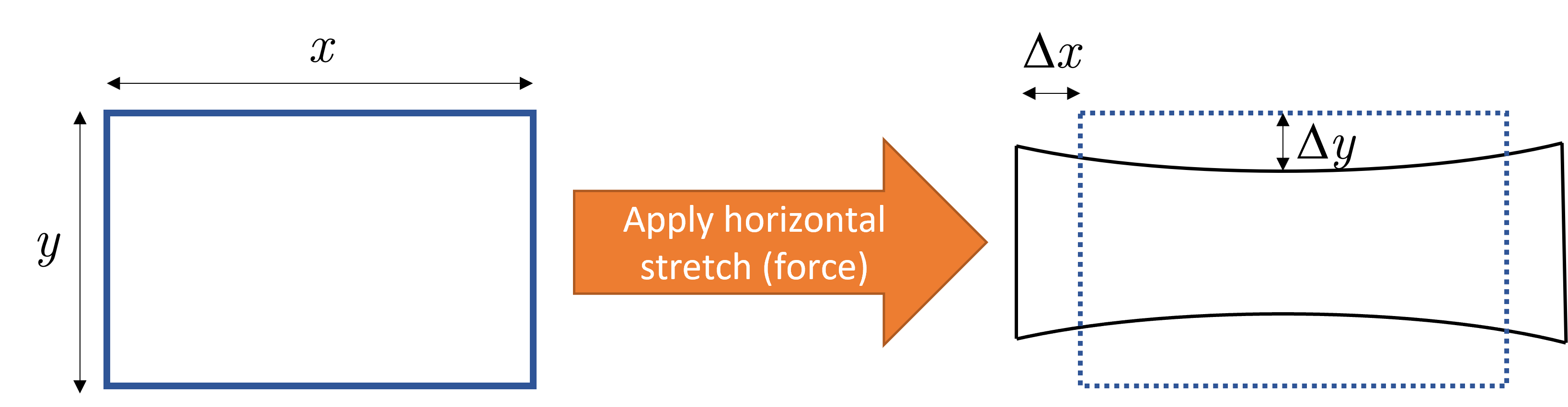
$A horizontal force is applied to a material such that it is stretched along the $x$ direction. The length parallel to the stretch increases by $\Delta x$ and the width (i.e. along $y$ axis) changes by $\Delta y$. For positive $\nu$ the width decreases meaning the block of material gets thinner. For $\nu=0$ the width does not change and for auxetic materials ($\nu<0$) the material gets wider when stretched!$

Fig. 6 A horizontal force is applied to a material such that it is stretched along the $x$ direction. The length parallel to the stretch increases by $\Delta x$ and the width (i.e. along $y$ axis) changes by $\Delta y$. For positive $\nu$ the width decreases meaning the block of material gets thinner. For $\nu=0$ the width does not change and for auxetic materials ($\nu<0$) the material gets wider when stretched!#

We define Poisson’s ratio as the ratio of lateral strain $\varepsilon_{yy}$ and longitudinal strain $\varepsilon_{xx}$

(5)#\[\nu = \frac{-\varepsilon_{yy}}{\varepsilon_{xx}}= \frac{-\Delta y}{y}\frac{x}{\Delta x}\]

where the minus sign is included as $\Delta y$ was considered to be inherently negative when equation (5) was first defined. This is because most typical materials get thinner when stretched, and so the minus sign was included, I presume, to ensure that the ratio is positive. It is therefore possible to have a negative Poisson ratio if the material expands laterally under longitudinal strain. Such materials are known as auxetic materials and include foams, graphene, paper and tendons!
However for most materials the Poisson ratio is positive. An incompressible material has $\nu=0.5$, most ordinary solids have $\nu \approx 0.25-0.35$, and rubber behaves as if it were nearly incompressible ($\nu \lessapprox 0.5$).

Combining moduli with Poisson’s ratio#

Finally it is possible to derive relationships between elastic moduli (Young’s modulus, shear modulus and bulk modulus [not covered in this course] ) and Poisson’s ratio. It’s beyond the scope of this course to derive them explicitly but for reference the relationship involving the two moduli covered above is

(8)#\[G = \frac{Y}{2(1+\nu)}\]

If you are particularly interested in the fine details of elastic moduli and Poisson’s ratio, and in particular how they are all interrelated then I recommend taking a look at section 4.2 in the book by Sadd [2014]. You do not need to understand the material in the textbook for this module - this is only for those who want a deeper understanding.

Shearing a liquid - stress and strain rate.#

So far we have spent a lot of time exploring how solids respond to an applied shear stress. It logically follows that we should consider what happens to a liquid when a similar shear stress is applied. So let us crack on.

Let us return to the schematic shown in Fig. 5 but this time we have a liquid occupying the grey region between the two plates. When a shearing force $\sigma$ is applied to the top plate the fluid flows meaning we need to consider the velocity of the fluid between the plates. Unfortunately the system for a liquid flowing is a little more complicated compared to a solid being deformed, but we can use the definition for shear strain (equation (2)) to help.

The layer of liquid immediately touching the top plate will flow with a velocity $v$ but the layer touching the bottom plate will remain stationary. This means that we have a velocity gradient through the material that is linear for simple liquids, or that the velocity is proportional to the vertical distance $y$ from the stationary plate and we shall use a temporary constant of propotionality $\zeta$ so that we can state

\[\begin{align*} v &= \zeta y, \text{ or}\\ \zeta &= \frac{v}{y} \end{align*}\]

Remember though that the velocity here is the horizontal velocity, meaning that $v = \dfrac{\mathrm{d}x}{\mathrm{d}t}$. So

\[\begin{align*} \zeta &= \frac{\mathrm{d}x}{\mathrm{d}t}\,\frac{1}{y}\\ &= \frac{\mathrm{d}}{\mathrm{d}t}\left(\frac{x}{y}\right) = \dot{\gamma} \end{align*}\]

This means that when a shear stress $\sigma$ is applied to a liquid there is a flow quantified by and proportional to the shear strain rate. For a solid we introduced a constant of proportionality ($G$) that may have been unfamiliar to you, but for a liquid this constant of proportionality is much more familiar; it is the viscosity $\eta$.

Viscosity being the constant of proportionality should make sense here. A liquid with a high viscosity does not readily flow under a given force whereas a thin liquid (low viscosity) will flow more easily.

Viscoelastic materials.#

So far we have considered elastic solids and viscous liquids, and how we can distinguish between them. Applying a shear stress to a solid produces a constant shear strain, whereas a shear stress on a liquid produces a constant shear strain rate.
But what about those materials that falls somewhere inbetween? Silly putty and oobleck (cornflour in water) can flow as a liquid but also respond like an elastic solid when you strike them - these materials are known as viscoelastic materials.. The key observation is that the mechanical properties of viscoelastic materials depend on the timescale in which the deformation is applied.

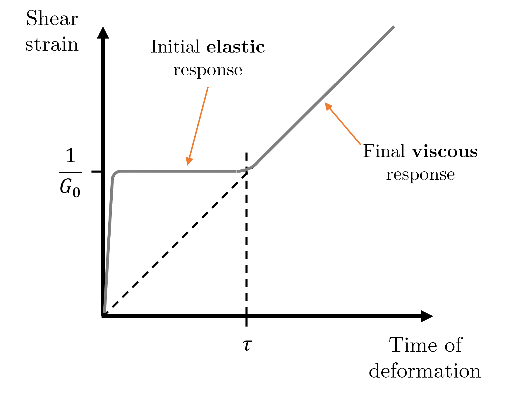
$A constant shear stress is applied to a viscoelastic material at $t=0$. At short timescales ($t<\tau$) the material exhibits elastic-like behaviour, namely that there is a constant shear strain in the material. For longer timescales the material flows and the shear strain changes with time - in this example the strain rate is constant giving a linear response for $t>\tau$.$

Fig. 7 A constant shear stress is applied to a viscoelastic material at $t=0$. At short timescales ($t<\tau$) the material exhibits elastic-like behaviour, namely that there is a constant shear strain in the material. For longer timescales the material flows and the shear strain changes with time - in this example the strain rate is constant giving a linear response for $t>\tau$.#

Consider Fig. 7. When a stress is applied over a short timescale (such as hitting the material) it behaves like an elastic solid, with an instantaneous shear modulus $G_0$. After some characteristic relaxation timescale $\tau$ the material begins to flow.
This allows us to define a scaling relationship between $\tau$, $G_0$ and $\eta$. The gradient of the viscous region is inversely proportional to the viscosity (more viscous means less flow meaning lower shear strain rate). We then extrapolate back from the transition point at $t=\tau$ which gives a gradient of the dashed extrapolation line of $\dfrac{1}{G_0\tau}$, and as both the extrapolation and viscous response domain have the same gradient we can state that

(9)#\[\eta\sim G_0\tau\]

We call this a scaling relationship because it describes the relationship between the different parameters but there may be an additional numerical parameter unknown to us. We hope that this numerical prefactor is of order unity but either way the scaling relationship argument provides us with a starting point from which to construct more accurate models.

Although ‘typical’ (i.e. Newtonian) fluids follow a linear relationship between stress and strain rate, there are other fluid systems whose effective viscosity follow a non-linear relationship between strain rate and stress. These non-Newtonian fluids broadly fall under two categories:

Shear thinning - increased strain rate reduces the effective viscosity (gets thinner with more strain applied per unit time),
Shear thickening - increased strain rate increases the effective viscosity (gets thicker with more strain applied per unit time). Some schematics of Newtonian (a), shear thinning non-Newtonian (b) and shear thickening non-Newtonian (c) fluids can be found in Fig. 8.

$Stress-strain rate (left) and strain rate-effective viscosity plots for a) Newtonian, b) shear thinning and c) shear thickening liquids. A Newtonian liquid is defined as one where $\sigma \propto \dot{\gamma}$, with a constant of proportionality $\eta$, i.e the viscosity. A non-Newtonian liquid shows a non-linear relationship between $\sigma$ and $\dot{\gamma}$, and consequently the effective viscosity depends on the strain rate i.e. $\eta(\dot{\gamma})$$

Fig. 8 Stress-strain rate (left) and strain rate-effective viscosity plots for a) Newtonian, b) shear thinning and c) shear thickening liquids. A Newtonian liquid is defined as one where $\sigma \propto \dot{\gamma}$, with a constant of proportionality $\eta$, i.e the viscosity. A non-Newtonian liquid shows a non-linear relationship between $\sigma$ and $\dot{\gamma}$, and consequently the effective viscosity depends on the strain rate i.e. $\eta(\dot{\gamma})$#

These types of behaviours have been observed and experimentally studied for a long time, but can we understand what is going on at the molecular level that would give rise to these different macroscopic behaviours. We can make some initial assumptions about the systems, particularly the instantaneous shear modulus $G_0$ and relaxation time $\tau$, from which we can build our theoretical constructs.

The instantaneous shear modulus will likely depend on the forces between individual molecules. We would not expect this to depend strongly on temperature.
The relaxation time arises from the way that molecules can move around themselves and one another. We expect there to be a strong temperature dependence given that the motion of molecules is a statistical / thermodynamic process.

So now that we’ve got a starting point, let us jump straight in to the details!

Moduli and relaxation times at the atomic level.#

Shear modulus - calculating from first principles#

For the purposes of simplicity we are going to calculate the Young’s modulus from first principles. It is possible to also calculate other moduli using similar arguments but they also introduce some extra geometry that makes it more complicated without adding anything to the conceptual understanding of what is going on.

We start by assuming that we have a cuboid block of material of initial length $L$ and cross sectional area $A$. A force $F$ is applied along the length such that the block length increase by $\Delta L$.
Next we zoom in to the atomic level as shown in Fig. 9.

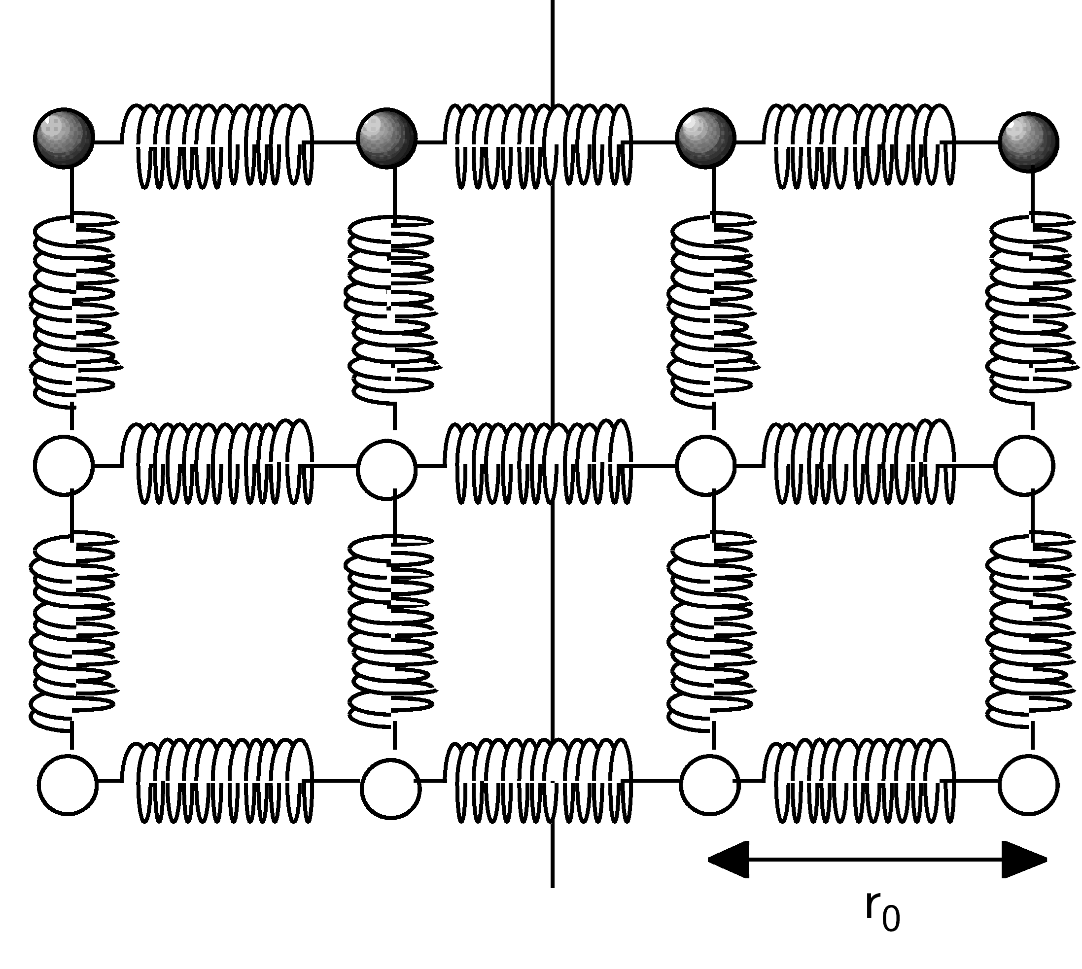
Fig. 9 Ball and spring model of a solid. At equilibrium each atom is a distance $r_0$ from its nearest neighbour.#

Here we model our solids as a collection of spheres (the atoms) and springs (the interatomic forces) arranged in a simple cubic structure that aligns with the edges of the macroscopic block of material. When there is no force applied to the block each of the atoms are separated by a distance $r_0$, and applying the force $F$ causes the springs aligned in the direction of $F$ (in this case we will call this the $x$ direction) to extend to a new legth $r$. The springs are assumed to obey Hooke’s law such that $F=k(r-r_0)$ and each atom has an effective cross sectional area of $r_0^2$ in the $y,z$ plane.
Thus the associated stress is

(10)#\[\sigma_{\text{tensile}} = \frac{F}{r_0^2} = \frac{k(r-r_0)}{r_0^2}\]

The strain experienced by each atom as a result of the applied stretching force is

(11)#\[\varepsilon_{\text{tensile}} = \frac{r-r_0}{r_0}\label{eq:C1_YoungSpring2}\]

and by combining equations (10) and (11) we find the Young’s modulus to be

(12)#\[\begin{split}Y &= \frac{k(r-r_0)}{r_0^2}\frac{r_0}{r-r_0}\\ &= \frac{k}{r_0}\label{eq:C1_YoungSpring3}\end{split}\]

In the classical macroscopic treatment we would normally stop here and accept that the spring constant $k$ is some inherent parament of the spring. Here however we are modelling the interatomic forces and energies as a spring, and it would be more insightful to move away from $k$ into a model that relates to interatomic energies.
We can approximate the interatomic potential $U$ around the equilibrium separation $r_0$ by treating it like a harmonic oscillator, and so

\[\begin{align*} U(r) &= U(r_0) + \frac{1}{2}(r-r_0)^2\frac{\mathrm{d}^2U}{\mathrm{d}r^2}\bigg\rvert_{r=r_0}+\text{ higher order terms}\\ &= \text{constant} + \frac{1}{2}k(r-r_0)^2 \end{align*}\]

where the first line is a Taylor expansion for a harmonic oscillator and the second line is the potential energy of a spring that includes some constant zero offset. The particular form of the interatomic potential depends on the actual system at hand but we can generalise it as

\[\begin{align*} U(r) &= \epsilon\,f\left({\scriptstyle \frac{r}{r_0}}\right) \end{align*}\]

where the potential has a miminum value of $-\epsilon$ at $r=r_0$ (i.e. the bond energy), and so $f(\frac{r}{r_0})$ is a dimensionless function that satisfies the condition $f(1) = -1$. Using this general function with the above approximation for the interatomic potential we find that

\[\begin{align*} k = \frac{\mathrm{d}^2U}{\mathrm{d}r^2}\bigg\rvert_{r=r_0} = \frac{\epsilon}{r_0^2}\,f''(1) \end{align*}\]

where $f''(1)$ is a dimensionless number. The value of this number depends on the actual form of the potential involved but for the sake of simplicity we will generalise this to say that $f''(1)=B.$. Therefore equation (12) becomes

(13)#\[Y = B\frac{\epsilon}{r_0^3}\]

Let us take a moment to pause and reflect on what equation (13) is actually telling us. This simple model predicts that the rigidity of a material (a macroscopic property) depends on the \textbf{bond density} at the interatomic level. A rigid material will have either strong interatomic bond strength, shorter interatomic spacing, or, more likely, some combination of the two. This feels right intuitively but it’s always nice to see it fall out from a structured argument.

Relaxation time, viscosity, and temperature dependence.#

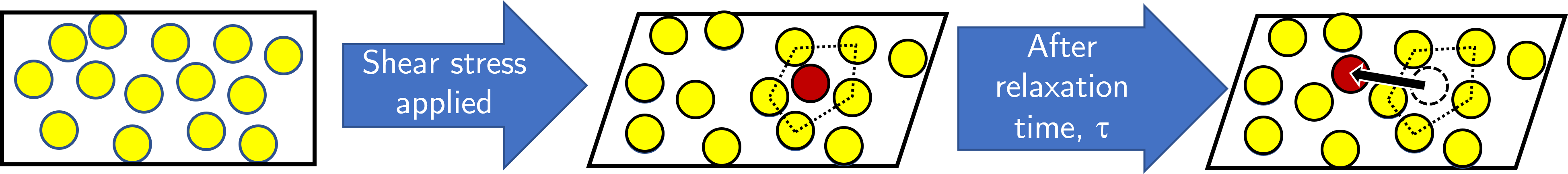
$A liquid is initially at rest (left) and then a shear stress is applied that causes some of the atoms (labelled red) to be closely surrounded by and intereacting more with neighbouring molecules (centre figure). After some characteristic time $\tau$ the atom is able to escape the cage and move to a region of lower free energy.$

Fig. 10 A liquid is initially at rest (left) and then a shear stress is applied that causes some of the atoms (labelled red) to be closely surrounded by and intereacting more with neighbouring molecules (centre figure). After some characteristic time $\tau$ the atom is able to escape the cage and move to a region of lower free energy.#

We can now turn out attention to more complex liquids that are subjected to some applied stress. On the left hand side of figure Fig. 10 the liquid is represented by a black box and is made up of individual yellow molecules. These molecules do not have any long range order and the interatomic / intermolecular distance is a range rather than a single value (some are closer together, others further apart). We then apply some shear stress such that the liquid deform (middle figure). In doing so the individual atoms or molecules are also moved and in some cases an atom or molecule, highlighted in red, finds itself much closer to its neighbours than would be expected in the unsheared case. These reduced distances means that the total interaction energy of this atom / molecule is high, and the system will want to change in order to minimise the energy of the system. We find that after some characteristic time $\tau$ the ‘trapped’ molecule is able to escape the ‘cage’ formed by the too-close neighbours and relaxes into a new position that reduces the energy of interaction between that atom or molecule and the new neighbours.

Sounds logical. But can we construct some logical argument that allows us to quantify $\tau$ in terms of other properties of the system, such as the temperature or interaction energy? Of course, otherwise this would be a short and pointless section!

We start our argument by recognising that the trapped molecule is not simply sitting there waiting until it is time to hop out of the cage. Instead the molecule will be continuously vibrating within the cage, moving with a continuously changing that depends on the thermal energy of the molecule and the interaction energy between neighbours $\epsilon$. What we have here is a statistical mechanics system, meaning we are interested in the probability that the molecule will be able to escape the cage by overcoming the energy barrier $\epsilon$ and that this probability is given by the Boltzmann distribution. Thus the characteristic time to escape the cage is

(14)#\[\tau^{-1} \sim \nu\,\, \text{exp}\left(-\frac{\epsilon}{k_\text{B}T}\right)\]

The exact values for $\nu$ and $\epsilon$ will depend on the material we are studying but from a conceptual perspective we can get some understanding if we make some reasonable estimates about these parameters. As an order of magnitude argument is only what we are interested here, we assume that the frequency $\nu$ is comparable to that of the frequency of phonons near the Brillouin zone boundary which are of order THz, or $10^{12}\text{ s}^{-1}$. We then note that the upper limit on the energy barrier $\epsilon$ must be the latent heat of vaporisation per molecule $\epsilon'$ otherwise the molecule escapes the liquid entirely as a vapour. Experimental data shows that for many simple liquids the approximation $\epsilon \approx 0.4\epsilon'$ is reasonable. Again we are interested in order of magnitudes so using the latent heat per molecule of water as $6.67\times10^{-20}\text{ J}$ means that $10^{-20}\text{ J}$ will suffice for a simple liquid.

Plugging in these order of magnitude values tells us that the relaxation time of a simple liquid is of order $10^{-12}-10^{-10}\text{ s}$.

Again let us stop here and think about the the implications of this, and to do so we should make reference back to Fig. 7. There are two important conclusions we can draw, one which is fairly straightforward but the other is perhaps a little surprising.

We can see that the relaxation time, i.e. the characteristic time at which a viscoelastic material ‘changes’ from elastic to viscous, depends on two parameters; $\nu$ which relates to the molecule itself and $\epsilon$ that characterises the interaction between the molecule and its neighbours. So a viscoelastic material that has a long relaxation time will have molecules that, for reasons we will consider later, make fewer attempts to escape the cage or have a higher interaction energy with neighbouring molecules. The actual reason is somewhere between the two, but we will come back to this later in the course.

The second and more surprising outcome from equation (14) and the paragraph that follows is that water, for example, has a characteristic time $\tau$. The implication here is that water also behaves like a viscoelastic material but only if you were to observe the response to shear at the subnanosecond domain. You might wonder why this is the case, and again we look back to $\nu$ and $\epsilon$ - you might start to wonder why water and simple liquids have small $\tau$, and a reasonable hypothesis could be that the size of the molecule could play a part. Hold that thought for now.

Combining equations (9) and (14) gives

(15)#\[\eta = \frac{G_0}{\nu}\,\text{exp}\left(\frac{\epsilon}{k_\text{B}T}\right)\]

meaning that the viscosity of our viscoelastic material in the domain of $t>\tau$ varies exponentially with temperature. This is known as an Arrhenius form, named after the more common version in physical chemistry that gives an empirical model of how the rate constant of a chemical reaction depends on temperature.

Unfortunately this is not the end of the story. Some liquids do indeed follow an Arrhenius behaviour whereas others show what some call a “super-Arrhenius” type behaviour. The temperature dependence of viscosity in these liquids is much stronger than a simple exponential behaviour. Consider Fig. 11.

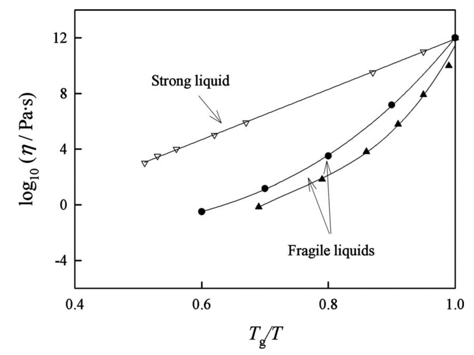
Plot of normalised temperature against log of viscosity. A linear dependence is found for strong liquids (such as silicon dioxide, labelled by open triangle) whereas fragile liquids (glycerol (solid circles) and sucrose (solid triangles) do not show a linear relationship.

Fig. 11 There are some liquids, known as strong liquids, whose viscosity-temperature depenence follows the Arrhenius form given in equation (15). Other liquids are more complex and show a non-linear relationship between $\ln \eta$ and $T^{-1}$ - these liquids are sometimes called fragile liquids.
Care needs to be taken with the horizontal axis. It is normalised such that unity refers to the temperature at which the liquid becomes rigid (glass - see next section) and values below 1 are temperatures above this glass temperature.
The strong liquid (open triangles) is $\text{SiO}_2$ whereas the fraile liquid are glycerol (solid circles) and sucrose (solid triangles). Figure from Longinotti and Corti [Longinotti and Corti, 2008]#

The axes in this figure are a typcial choice for studying the temperature dependence of viscosity. From equation (15) it follows that plotting $\ln \eta$ against $\frac{1}{T}$ should give a straight line with gradient equal to $\dfrac{\epsilon}{k_\text{B}}$ and intercept $\dfrac{G_0}{\nu}$. Therefore any data that lies on a straight line on these axes is a liquid that shows Arrhenius-type behaviour. By plotting data from three different liquids in Fig. 11 we immediately see that one of them shows Arrhenius-type behaviour associated with a simple liquid (in this case, $\text{SiO}_2$) but two different sugars show a much stronger temperature dependence and are consquently not a simple liquid. Some authors call these fragile liquids though this terminology is not used by everyone.

Now, remember not long ago I told you to hold that thought? Here we have some experimental data that does support our intuition that the size of the molecules may play a part in whether a liquid is simple or not. $\text{SiO}_2$ is a relatively small molecule whereas sucrose ($\text{C}_{12}\text{H}_{22}\text{O}_{11}$) is much larger - in terms of molar mass, sucrose is 6 times more massive. The two molecules are also rather different in shape too but that is something we will explore in much more detail in Topic 2.

Even putting aside the fine detail regarding the role of molecule size and shape we can still gain some insight into the possible causes of the non-Arrhenius behaviour exhibited by some liquids and what happens to these materials when we cool them to a rigid but non-crystalline state known as a glass.

Bibliography#

LC08: M. Paula Longinotti and Horacio R. Corti. Viscosity of concentrated sucrose and trehalose aqueous solutions including the supercooled regime. Journal of Physical and Chemical Reference Data, 37(3):1503, jul 2008. URL: https://aip.scitation.org/doi/abs/10.1063/1.2932114, doi:10.1063/1.2932114.
Sad14: Martin H. (Martin Howard) Sadd. Elasticity : theory, applications, and numerics. Elsevier, Amsterdam, third edition. edition, 2014. ISBN 0-12-410432-0.