3.2 - Liquid-liquid unmixing

3.2 - Liquid-liquid unmixing#

Equilibrium phase diagrams.#

In this example we are going to consider to partially miscible liquids that are mixed at high temperatures but unmix at lower temperatures. We consider partially miscible because we want to understand the phase transition of two liquids A and B from mixed to unmixed or vice versa (shown in Fig. 44), in particular in understanding the free energy of these states.

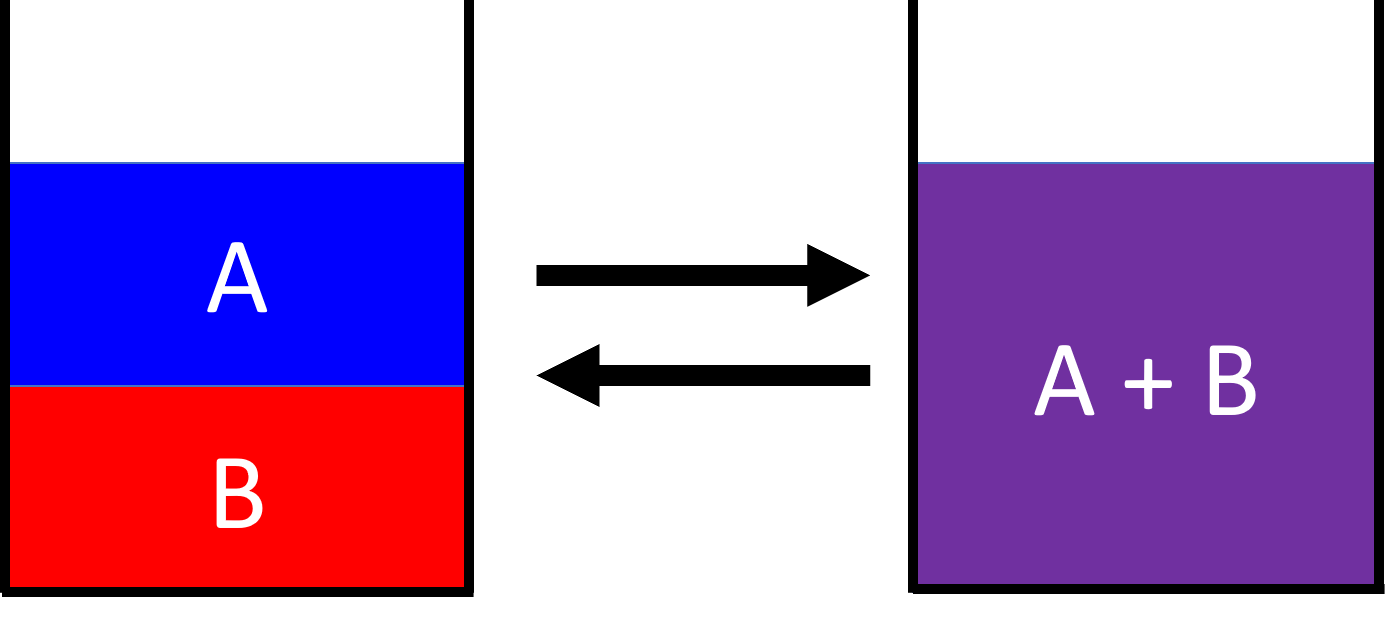
Fig. 44 A system comprised of two liquids A and B that are either unmixed (left) or completely mixed (right).#

In the unmixed state the total free energy is equal to the sum of the free energies for the two phases, i.e. $F_A+F_B$. If the free energy of the mixed state is $F_{A+B}$ then the free energy of mixing is

\[F_{mix} = F_{A+B}-(F_A+F_B)\]

and if we can predict how $F_{mix}$ changes with respect to the change in entropy and energy on mixing, $S_{mix}$ and $U_{mix}$ respectively, we can predict the phase behaviour of our liquids.

First we will consider the entropy of the system. To do this we are going return to the idea of constraining our molecules to a lattice (see Fig. 28 for example). In Fig. 45 the liquids are mixed and sites are occupied by either an A or B molecule.

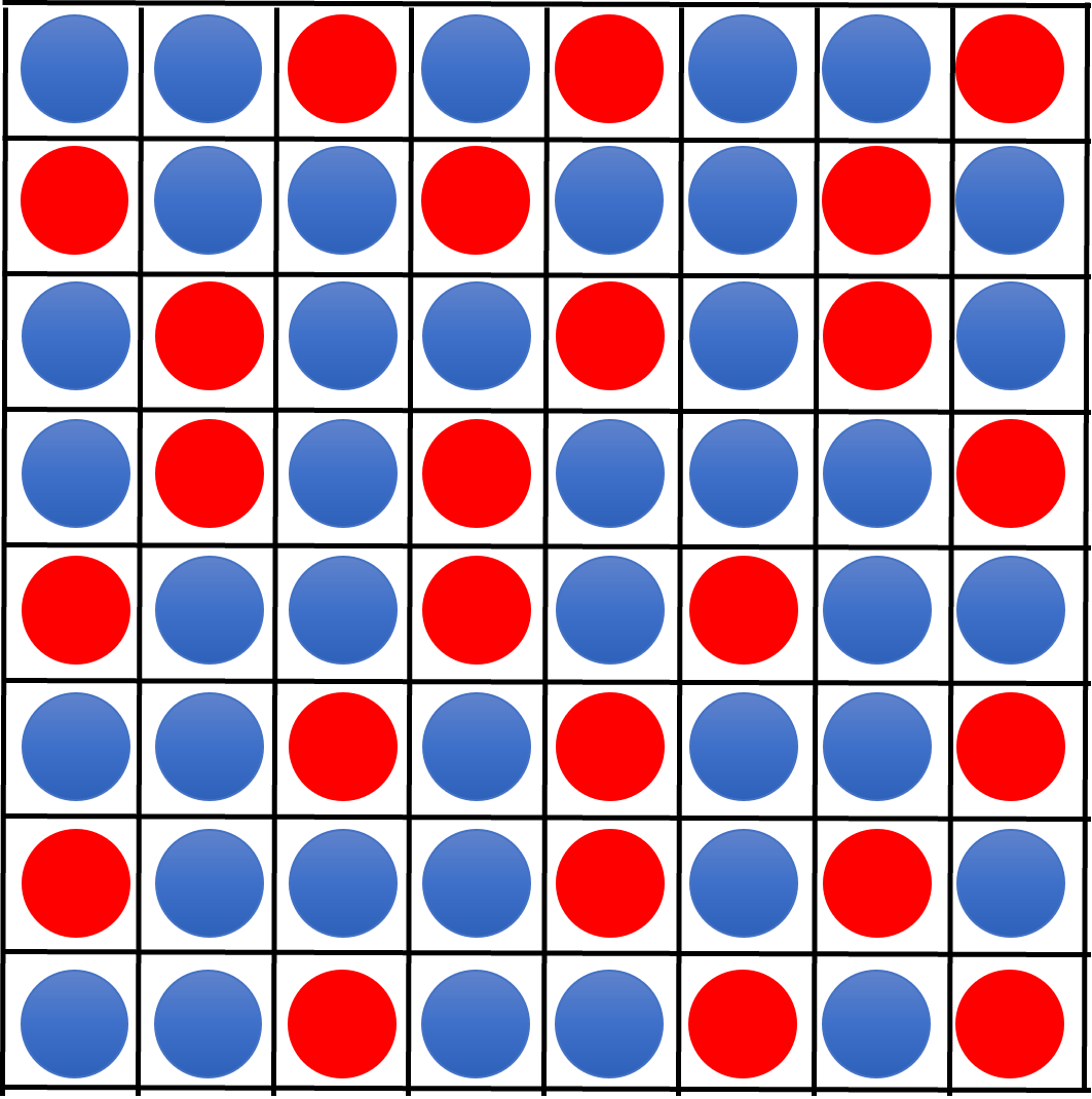
A lattice model of a mixed liquid-liquid system. Despite using a lattice model we are not assuming there is any long range order in the system. The lattice acts as a tool to simplify how we identify and count neighbouring interactions.

Fig. 45 A lattice model of a mixed liquid-liquid system. Despite using a lattice model we are not assuming there is any long range order in the system. The lattice acts as a tool to simplify how we identify and count neighbouring interactions.#

We can consider the concentration of molecules in terms of the volume fractions $\phi_A$ and $\phi_B$ where we assume the volume of each molecule is the same. If the material is incompressible then $\phi_A+\phi_B=1$.
The lattice shown in Fig. 45 is just a sample ‘snapshot’ of the system; in reality we do not know whether a given site on the lattice is occupied by an A or B molecule, but we do know it must be one or the other. This allows us to use some statistical mechanics, namely the Boltzmann equation

\[S=-k_\text{B}\sum_ip_i\ln p_i\]

where $p_i$ is the probability that a lattice site is in a particular state $i$, which in our case is either A or B. Thus the entropy of mixing per site is

\[\begin{split}S_{mix} &= -k_\text{B}\left(p_A\ln p_A + p_B\ln p_B\right)\\ &= -k_\text{B}\left(\phi_A\ln \phi_A + \phi_B\ln \phi_B\right)\end{split}\]

where the probabilities are equal to the volume fractions because the total volume $V$ is constant.

But what about the energy of mixing? We’ve actually already covered the concepts behind defining this change in energy when we discussed the $\Theta$ temperature. Instead of considering a polymer-solvent interaction we now need to think about A-B interactions.

Looking at our lattice again there are three types of energy interactions between neighbouring sites. Two of these are for similar molecules, i.e. AA and BB, and the third is for different molecules AB. The interaction energy for each of these is thus $\epsilon_{AA}$, $\epsilon_{BB}$ and $\epsilon_{AB}$ respectively.

We use a mean field assumption that everything looks roughly the same across the whole mixed solution, meaning there are no local fluctuations. If each site has $z$ nearest neighbours then the interaction energy per site in the mixed state is

(51)#\[U_\text{fully mixed}= \frac{z}{2}\left(U_A\phi_A+U_B\phi_B\right)\]

where $U_A$ is the average interaction energy an A molecule would have at a given site, and is

\[U_A = \phi_A\epsilon_{AA}+\phi_B\epsilon_{AB}\]

and similarly

\[U_B = \phi_A\epsilon_{AB}+\phi_B\epsilon_{BB}\]

which means that equation (51) becomes

\[U_\text{fully mixed} =\frac{z}{2}\left(\phi_A^2\epsilon_{AA}+\phi_B^2\epsilon_{BB}+2\phi_A\phi_B\epsilon_{AB} \right).\]

In the completely unmixed state\footnote{Again, we ignore the interface between the unmixed volumes.} is

\[\begin{split}U_\text{unmixed} &= U_A + U_B\\ &= \frac{z}{2}\left(\phi_A\epsilon_{AA}+\phi_B\epsilon_{BB}\right)\end{split}\]

The total energy of mixing is thus the difference between the mixed and unmixed states above. This is

\[\begin{split}U_{mix} &= \frac{z}{2}\left[\left(\phi_A^2\epsilon_{AA}+\phi_B^2\epsilon_{BB}+2\phi_A\phi_B\epsilon_{AB} \right) - \left(\phi_A\epsilon_{AA}+\phi_B\epsilon_{BB}\right)\right]\\ &=\frac{z}{2}\left[\epsilon_{AA}(\phi_A^2-\phi_A)+\epsilon_B(\phi_B^2-\phi_B)+2\phi_A\phi_B\epsilon_{AB}\right]\end{split}\]

Remembering again that we assume the system is incompressible and only contains A and B molecules, then $\phi_A+\phi_B=1$. If we now only consider everything in terms of polymer A such that $\phi_A=\phi$ then $\phi_B = 1-\phi$ and so the expression for the interaction energy of mixing is

\[\begin{split}U_{mix} &= \frac{z}{2}\left[\epsilon_{AA}\left(\phi^2-\phi\right)+\epsilon_B\left((1-\phi)^2-(1-\phi)\right)+2\phi(1-\phi)\epsilon_{AB}\right]\\ &= \frac{z}{2}\left[\epsilon_{AA}\phi\left(\phi-1\right)+\epsilon_B\phi\left(\phi - 1\right)+2\phi(1-\phi)\epsilon_{AB}\right]\\ &= \frac{z}{2}\phi(1-\phi)\left[2\epsilon_{AB}-\epsilon_{AA}-\epsilon_{BB}\right]\\ &= \chi\phi(1-\phi)\end{split}\]

where $\chi$ is the Flory interaction parameter that we first saw back in equation (31) and is

\[\chi = \frac{z}{2k_\text{B}T}\left(2\epsilon_{AB}-\epsilon_{AA}-\epsilon_{BB}\right)\]

Bringing this all together means we can state the free energy of mixing per lattice site as

(52)#\[\begin{split}F_{mix} &= U_{mix}-TS_{mix}\\ &= \phi\ln\phi + (1-\phi)\ln(1-\phi) + \chi\phi(1-\phi)\\ [&=\phi_A\ln\phi_A + \phi_B\ln\phi_B + \chi\phi_A\phi_B]\end{split}\]

Equation (52) is, despite the simplicity of the expression, very powerful in describing how a liquid-liquid system will behave in terms of phase transitions. The two key terms here are the composition $\phi$ and the interaction parameter $\chi$, so we can seek to understand the phase behaviour by plotting the free energy for different $\phi$ and $\chi$ as shown in Fig. 46.

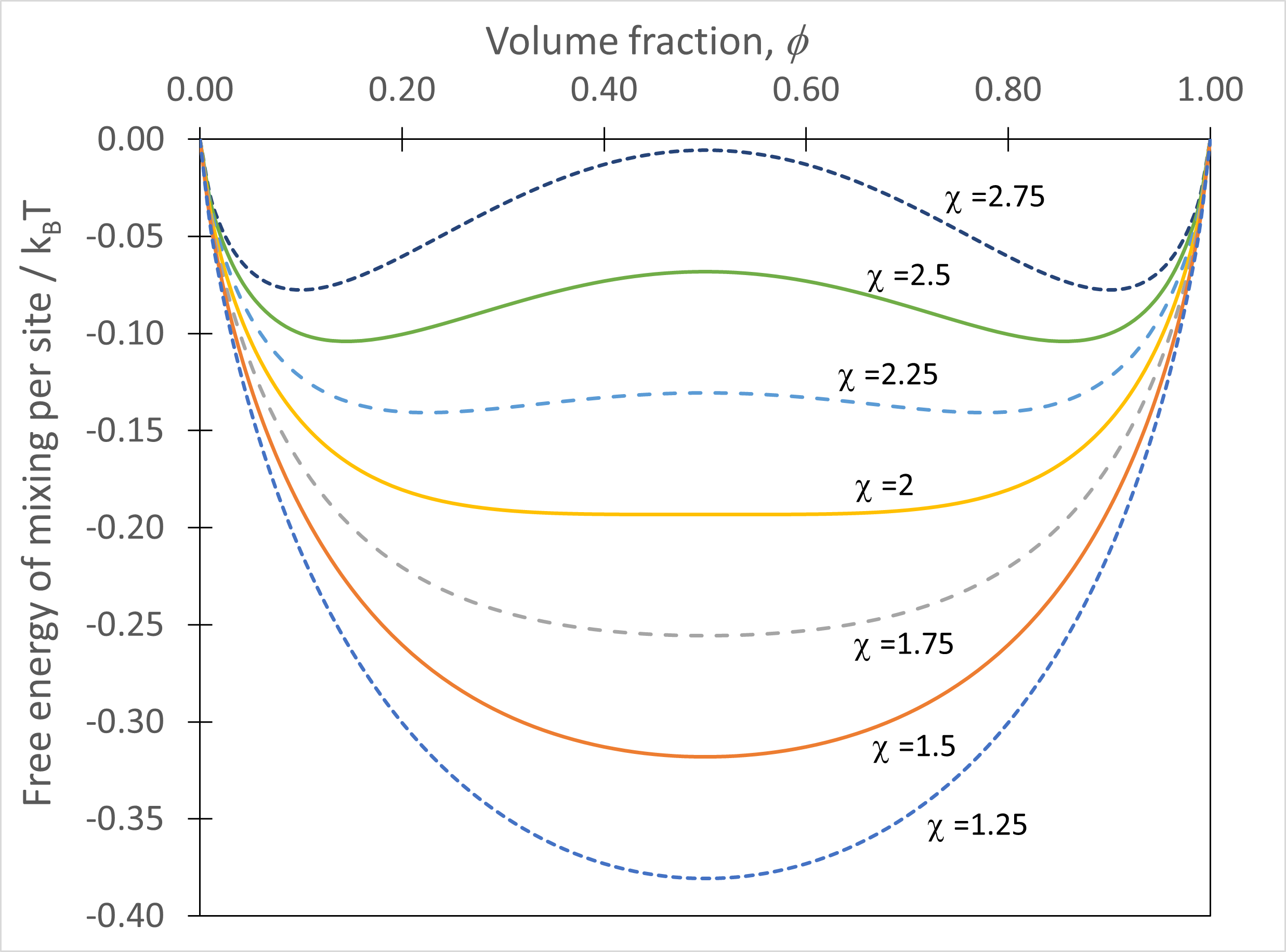
$Equation {eq}`eq:C3_Mixing` for simple molecular liquid-liquid system plotted as a function of volume fraction, with curves for different interaction parameters included.$

Fig. 46 Equation (52) for simple molecular liquid-liquid system plotted as a function of volume fraction, with curves for different interaction parameters included.#

For values of $\chi\leq2$ the curve has a single minimum at $\phi=0.5$ whereas for $\chi\geq2$ we find a maximum at $\phi=0.5$ and two minima either side of this.

Great, you’ve got a pretty graph with one bump or two. So what? Well we can interpret what these graphs mean physically if we consider how a physical system will behave in terms of a mixed versus unmixed states.

To do this we consider a volume $V_0$ whose starting volume fraction of molecule A is $\phi_0$. The mixture is then allowed to separate into two phases with volumes $V_1$ and $V_2$ and corresponding volume fractions of A $\phi_1$ and $\phi_2$. The process of unmixing would not change the total amount of A and B in the system, and so

\[\begin{split}\phi_0V_0 &= \phi_1V_1 + \phi_2V_2\\ \therefore \phi_0 &= \alpha_1\phi_1 + \alpha_2\phi_2\end{split}\]

where $\alpha$ is the relative proportion of the two phases, and consequently $\alpha_1+\alpha_2 = 1$. Thus the total energy of the phase-separate system is

\[\begin{split}F_\text{sep} &= \alpha_1F_{mix}(\phi_1)+\alpha_2F_{mix}(\phi_2)\\ &= \frac{\phi_0-\phi_2}{\phi_1-\phi_2}F_{mix}(\phi_1) + \frac{\phi_1-\phi_0}{\phi_1-\phi_2}F_{mix}(\phi_2)\end{split}\]

Interpreting this is insightful but not immediately obvious. The free energy at separation is related to the sum of the individual free energies of phases 1 and 2, which we expect. The prefactors to these free energies are a weighting term that considers the ‘distance’ between the unmixed and mixed compositions normalised by the total ‘distance’ between the two unmixed compositions. This is a little easier to see graphically in Fig. 47.

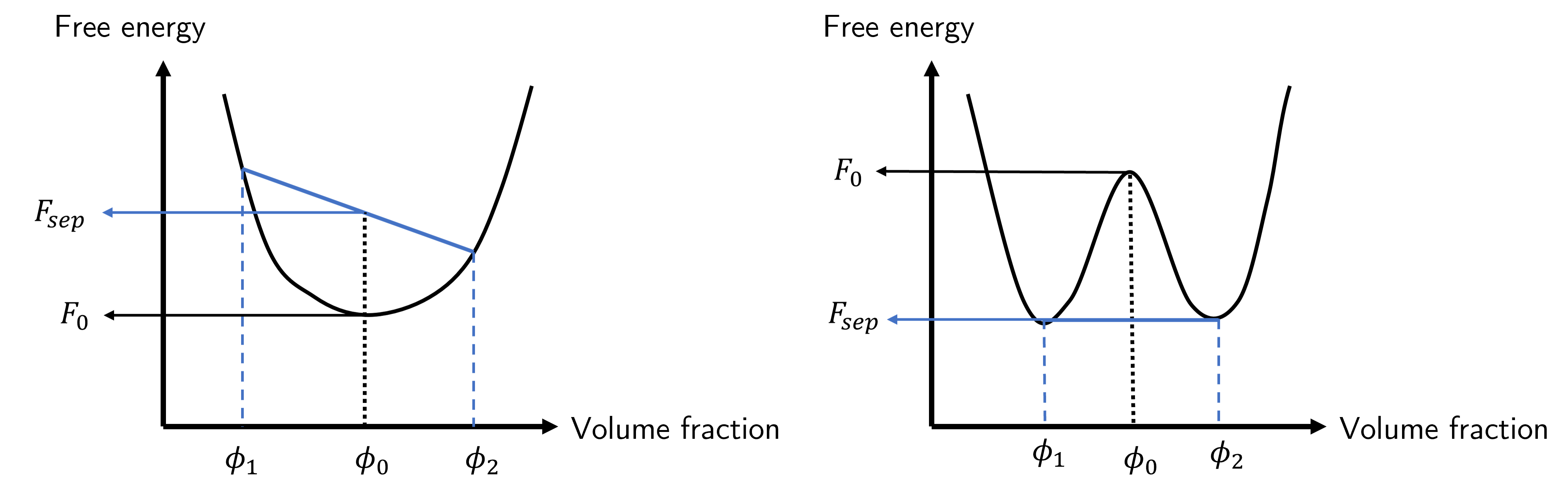
$Free energy curves for $\chi<2$ (left) and $\chi>2$ (right). The free energy of unmixing into two separate volume fractions $\phi_1$ and $\phi_2$ is compared to that at the mixed phase $\phi_0$.$

Fig. 47 Free energy curves for $\chi<2$ (left) and $\chi>2$ (right). The free energy of unmixing into two separate volume fractions $\phi_1$ and $\phi_2$ is compared to that at the mixed phase $\phi_0$.#

In this figure we can see the free energy of the mixed state $F_0$ (black) by simply finding the value of the curve when $\phi=\phi_0$. For the unmixed states we find the two free energies associated with the two compositions $\phi_1$ and $\phi_2$, and draw a line between the two free energies. We then find the value of the free energy on this line when $\phi=\phi_0$.\ In the case of the left hand curve of Fig. 47 we see that $F_0<F_\text{sep}$ which means the free energy of the mixed system is lower than the separated system, and consequently any unmixing would require additional energy. Remaining mixed is more energetically favourable meaning the system is stable.

Turning our attention to the right hand curve we see that, for the starting composition $\phi_0$ there are some compositions of an unmixed system that have a lower total free energy, and the one with the lowest possible free energy is formed when there is a common tangent at both points $\phi_1$ and $\phi_2$. These compositions are known as the coexisting compositions, and the line that is formed when the interaction parameter $\chi$ is changed (normally by changing the temperature) is known as the binodal or coexistence curve. We will come back to this shortly, but before then we need to think more deeply about the curvature of Fig. 47 as this will tell us about the local stability of a mixture.

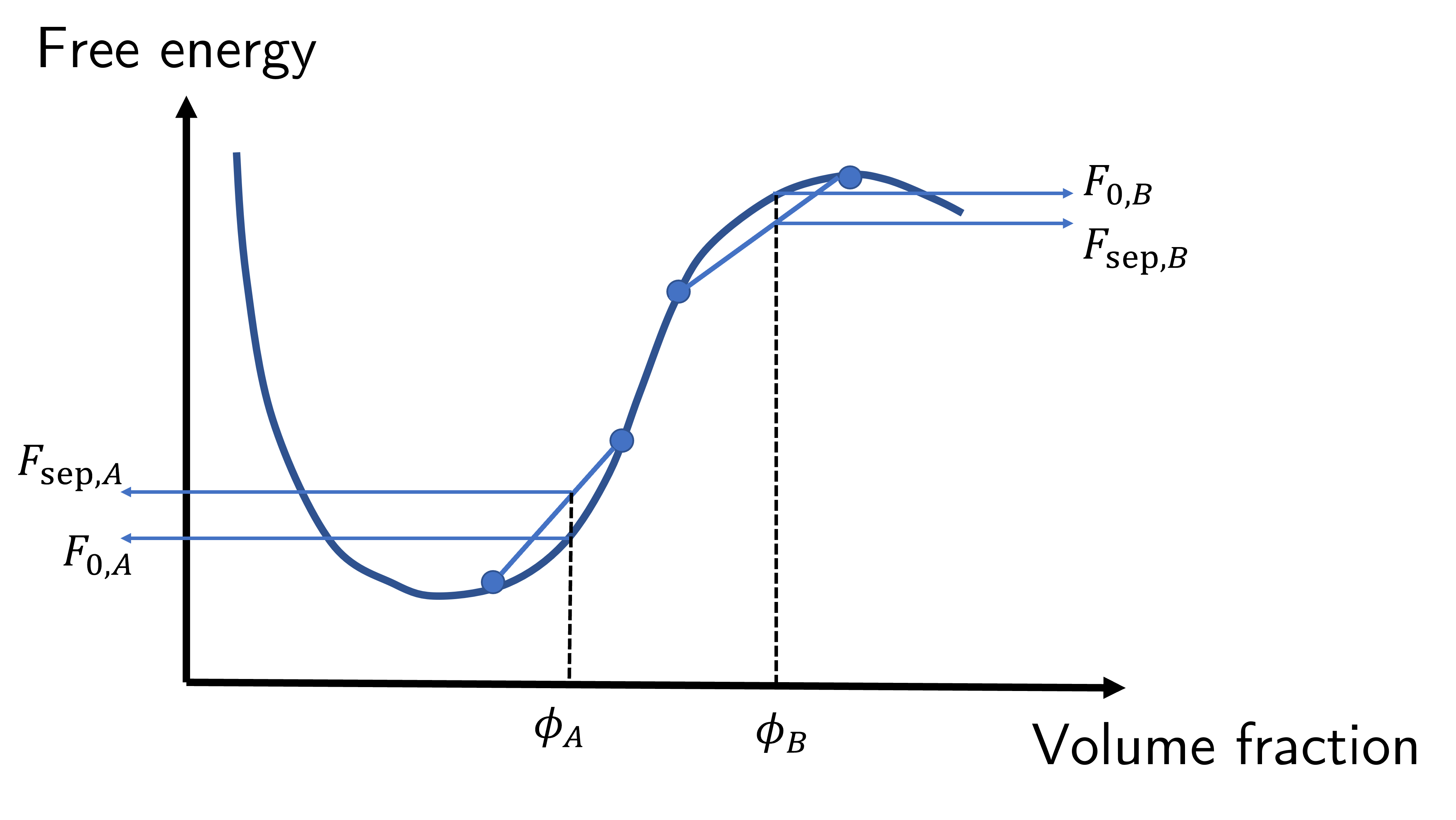
$Local stability is determined by the curvature of the free energy diagram. If the curvature is negative (around $\phi_B$) then the system is unstable, whereas a positive curvature (around $\phi_A$) is metastable.$

Fig. 48 Local stability is determined by the curvature of the free energy diagram. If the curvature is negative (around $\phi_B$) then the system is unstable, whereas a positive curvature (around $\phi_A$) is metastable.#

When the curvature $\dfrac{\mathrm{d}^2F}{\mathrm{d}\phi^2}$ is negative, such as the region about $\phi_B$ in Fig. 48 then the free energy due to separation is lower when the system locally separates out into two phases. All that is required is for a small local fluctuation to occur, which will occur due to the statistical nature of thermodynamics, that causes the system to phase separate. We would say that $\phi_B$ composition is unstable.

However for $\phi_A$ (i.e. when the curvature is positive) any small fluctuations in phases will increase the free energy and so even though $\phi_A$ does not have the lowest free energy possible, there needs to be a significant driving process to cause the system to phase separate; small scale fluctuations will not cause the system, but the system could phase separate out under the right conditions. As such we would call $\phi_A$ metastable.

Finally the condition when $\dfrac{\mathrm{d}^2F}{\mathrm{d}\phi^2}=0$ defines the boundary between meta- and unstable, and the locus of these points on a $\phi,\chi$ curve is known as the spinodal line. We can combine the spinodal and coexistence curves into a single phase diagram as shown in Fig. 49.

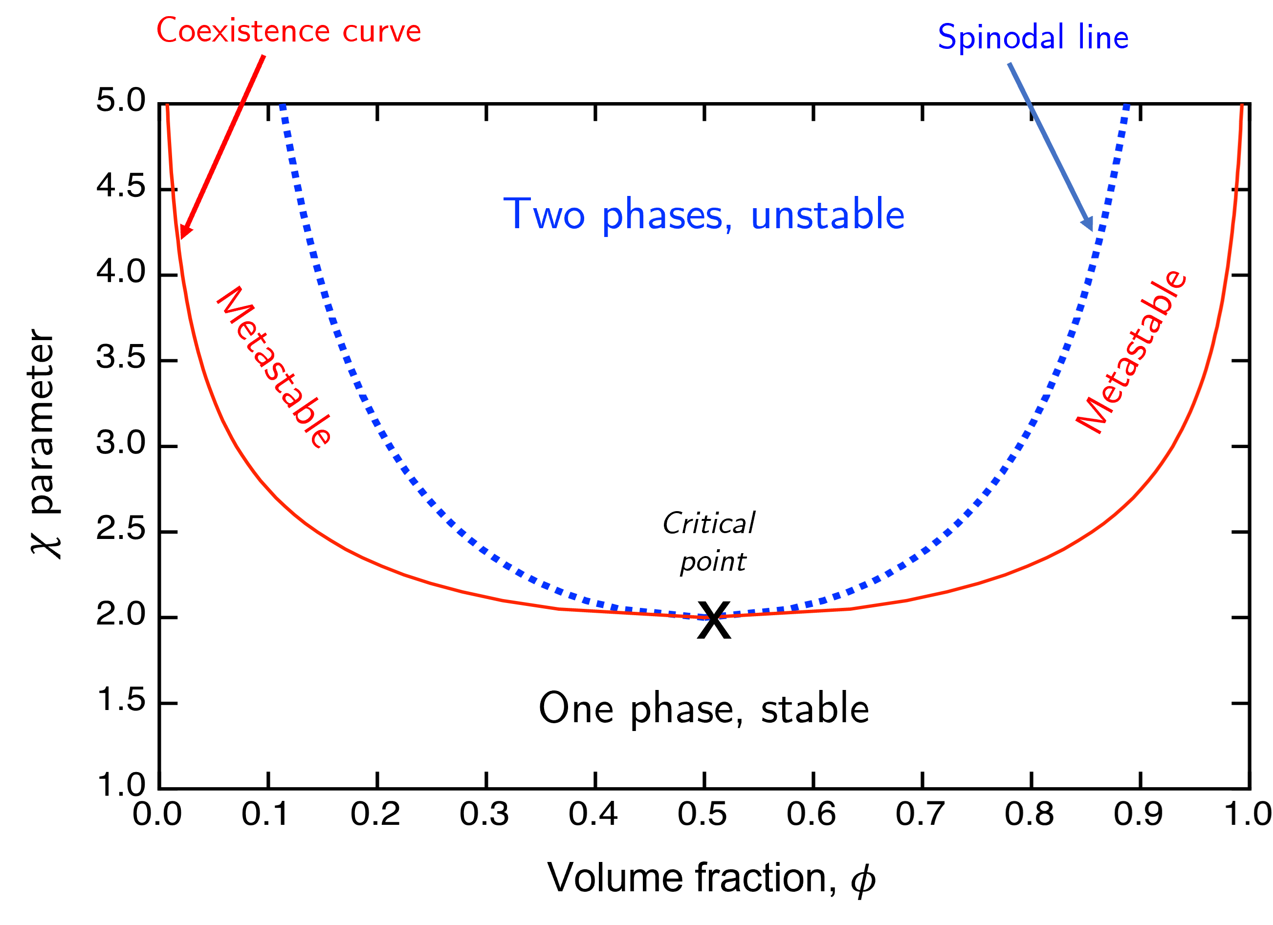
Fig. 49 A phase diagram for a simple molecular liquid-liquid system.#

Plotting these requires us to have a slightly more rigorous understanding of both the coexistence and spinodal lines, but we already have the starting points in the qualitative descriptions above.
For the coexistence curve we need to find a common tangent of the free energy at the compositions $\phi_1$ and $\phi_2$, which means

\[\left(\frac{\partial F_{mix}}{\partial \phi}\right)_{\phi=\phi_1} = \left(\frac{\partial F_{mix}}{\partial \phi}\right)_{\phi=\phi_2}\]

For the simple case of a symmetric lattice mixture (i.e. A and B are the same size) then the common tangent has gradient of zero, and so

(53)#\[\left(\frac{\partial F_{mix}}{\partial \phi}\right)_{\phi=\phi_1} = \left(\frac{\partial F_{mix}}{\partial \phi}\right)_{\phi=\phi_2} = k_\text{B}T\left[\ln\phi-\ln(1-\phi)+\chi(1-2\phi)\right) = 0\]

We can rearrange this to find the binodal $\chi_b$;

(54)#\[\begin{split}\chi_b &= \frac{1}{2\phi-1}\left(\ln\phi - \ln(1-\phi)\right)\\ &= \frac{1}{2\phi-1}\ln\left(\frac{\phi}{1-\phi}\right)\end{split}\]

which when plotted on the phase diagram in Fig. 49 gives the red (lower, solid) curve.

The spinodal line is found through

\[\frac{\partial^2 F_{mix}}{\partial \phi^2}=k_\text{B}T\left[\frac{1}{\phi}+\frac{1}{1-\phi}-2\chi\right] =0\]

from which we can solve to find the spinodal $\chi_s$;

(55)#\[\chi_s = \frac{1}{2}\left[\frac{1}{\phi}+\frac{1}{1-\phi}\right]\]

We can use this to find the critical point which is the point where the coexistence and spinodal curves meet. It is also the lowest point on the spinodal curve meaning

\[\frac{\partial \chi_s}{\partial \phi} = \frac{1}{2}\left[-\frac{1}{\phi^2}+\frac{1}{(1-\phi)^2}\right]=0\]

which occurs at $\phi = \frac{1}{2}$ in the case of a symmetric, molecular liquid. Plugging this in to equation (55) gives the critical interaction parameter $\chi_c=2$.

All of this has considered the phase behaviour of two molecular liquids. Now we will extend the system to consider a binary mixture of polymers, known as a polymer blend.

Mixing polymers - the polymer blend.#

Now instead of having two species A and B comprising of small molecules that each sit neatly in one lattice site, we now have two species of polymers with degree of polymerisation $N_A$ and $N_B$ respectively.

\[\frac{F_{mix}}{k_\text{B}T} = \frac{\phi}{N_A}\ln\phi + \frac{1-\phi}{N_B}\ln(1-\phi)+\chi\phi(1-\phi)\]

The good news is that we’ve already gone through the process once before to find the coexistence and spinodal curves, so all we need to do now is repeat the process but instead using the free energy of mixing for a polymer blend stated above. To simplify things a little we will consider only the symmetric case where $N_A = N_B = N$

For the coexistence curve we reuse equation (53) and find

\[\begin{split}\left(\frac{\partial F_{mix}}{\partial \phi}\right) &= k_\text{B}T\left[\frac{\ln\phi}{N}-\frac{ln(1-\phi)}{N}+\chi(1-2\phi) \right] = 0\\ \therefore \chi_b &= \frac{1}{(2\phi-1)N}\ln\left(\frac{\phi}{1-\phi}\right)\end{split}\]

Comparing this to equation (54) for a simple liquid we find that

\[\chi_{b, \text{blend}}=\frac{\chi_{b, \text{simple}}}{N}\]

We find a similar result for the spinodal

\[\chi_{s, \text{blend}} = \frac{1}{2N}\left[\frac{1}{\phi}+\frac{1}{1-\phi}\right] = \frac{\chi_{s,\text{ simple}}}{N}\]

The most important result here is that the critical interaction parameter also decreases by a factor of $N$, i.e.

\[\chi_{c, \text{ blend}} = \frac{\chi_{c, \text{ simple}}}{N} = \frac{2}{N}\]

and to understand why this is important we need to look back at Fig. 49. Notice that the critical interaction parameter is the lowest point on both the spinodal and coexistence curve and it also sets the upper value on $\chi$ for which all volume fractions are stable. As we increase the degree of polymerisation $N$ the critical value decreases, meaning the one phase / stable region on the phase diagram gets smaller and smaller.

This restricts the possible volume fractions in which a polymer blend can remain stable and, consequently, most polymers will not mix unless we can make $\chi\leq\frac{2}{N}$. Remembering that our simple model gives $\chi\propto T^{-1}$ this requires high temperatures for mixing to occur, and even then a small fluctuation will often cause phase separation to occur.

3.2 - Liquid-liquid unmixing

Contents

3.2 - Liquid-liquid unmixing#

Equilibrium phase diagrams.#

Mixing polymers - the polymer blend.#