2.4 Polymers: Back to macroscopic

2.4 Polymers: Back to macroscopic#

Rubber elasticity#

We have spent the past few sections considering polymers at the individual molecular level, and somewhat abstractly thought about how polymer chains behave in different concentrations. We can now take this knowledge of the molecular domain and see whether it can explain some of the macroscopic properties we covered at the start of the course when we examined shearing of different materials. We will first consider the elastic properties of rubber materials with the understanding that these materials are made up of many many polymer chains.

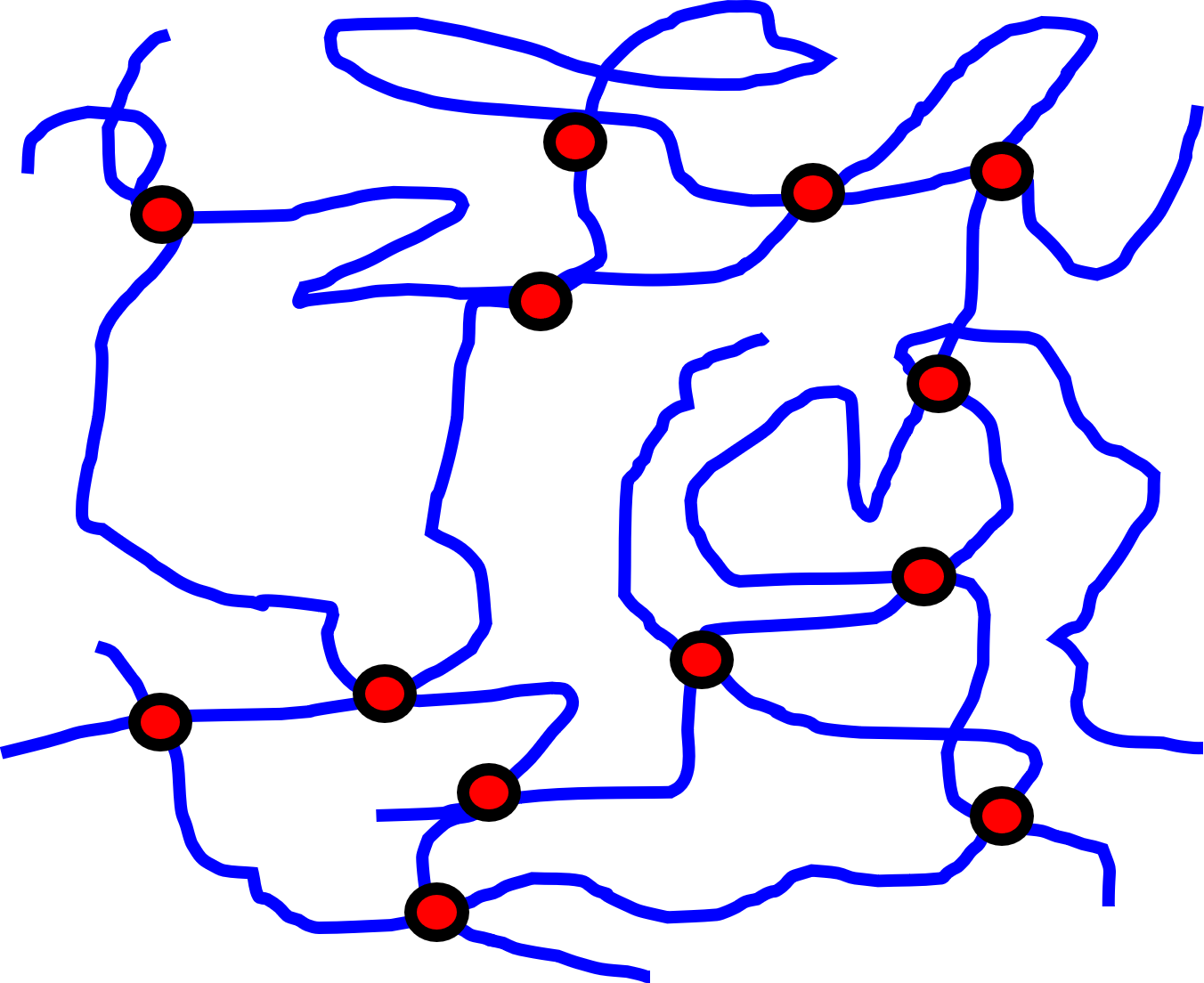
A conceptual model of a rubbery material. The rubber is made up of lots of polymer chains (blue lines) with crosslinks where chains cross over one another (red dots).

Fig. 33 A conceptual model of a rubbery material. The rubber is made up of lots of polymer chains (blue lines) with crosslinks where chains cross over one another (red dots).#

Start by assuming our rubber material is made up of polymer chains with $n$ crosslinks per unit volume (i.e. the crosslink density.) Fig. 33 provides a schematic of this, with the red dots indicating crosslinks in the system.

At this point we make use of the affine deformation assumption, which can be summarised as any linear transformation of the macroscopic material is also applied at the molecular level. So, if the sample dimensions change by some linear transformation

\[l_x,l_y,l_z \rightarrow \lambda_xl_x,\lambda_yl_y,\lambda_zl_z\]

then any point of a polymer chain will also transform by the same scales, i.e.

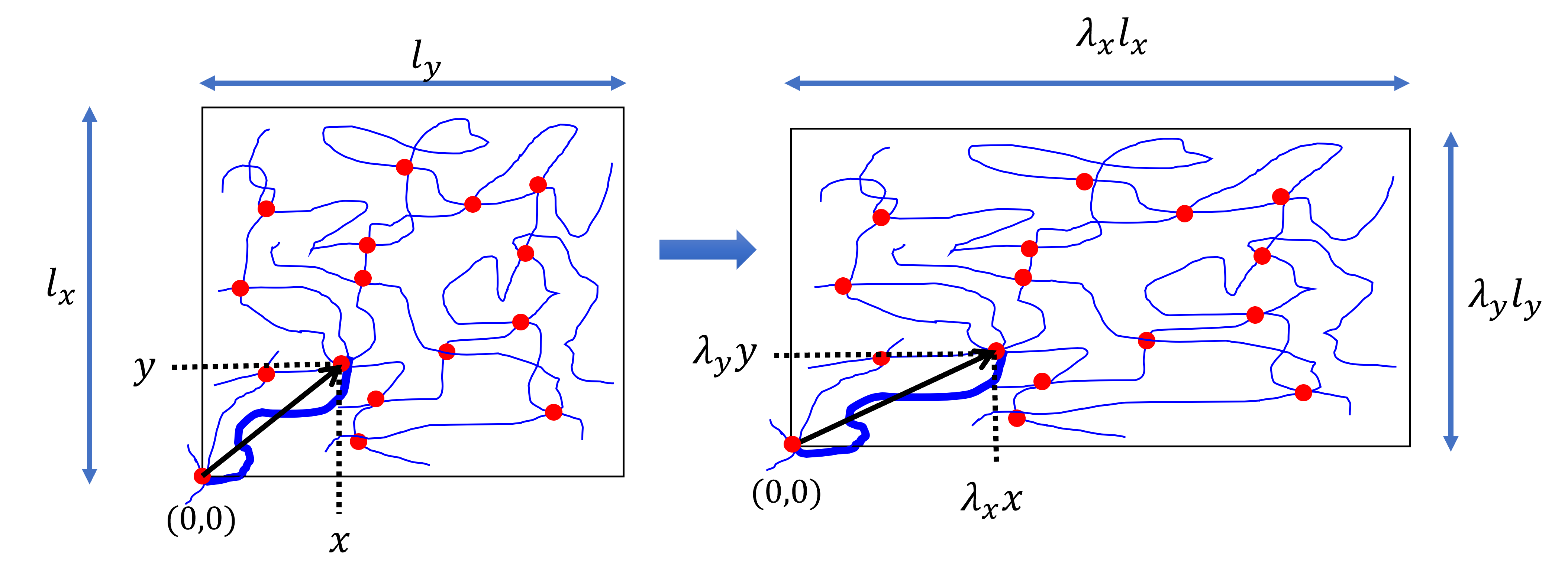
\[(x,y,z) \rightarrow (\lambda_xx,\lambda_yy,\lambda_zz)\]

The affine deformation assumption means that any linear transformation applied to the macroscopic material is 'replicated' at the molecular level. The thicker blue line is a single chain with one end fixed at the origin.

Fig. 34 The affine deformation assumption means that any linear transformation applied to the macroscopic material is ‘replicated’ at the molecular level. The thicker blue line is a single chain with one end fixed at the origin.#

Let us focus on a single polymer strand in the material. We shall fix one end of the chain at the origin (bottom left in Fig. 34, emphasised with a thicker line). The coordinate of the other end of the chain is $(x,y,z)$ and $(\lambda_xx,\lambda_yy,\lambda_zz)$ respectively, which allows us to calculate the original chain length $r_0$ as

\[r_0^2 = x^2+y^2+z^2\]

and the length after stretching is

\[r_1^2 = \lambda_x^2x^2 + \lambda_y^2y^2 + \lambda_z^2z^2\]

Recall that the entropy of a chain with length $r$ is

\[S(r) = -\frac{3k_\text{B}r^2}{2Na^2} + \text{constant}\]

and so the change in entropy due to stretching our rubber polymer chain is

(36)#\[\Delta S_\text{molecule} = -\frac{3k_\text{B}}{2Na^2}\left[\left(\lambda_x^2-1\right)x^2+\left(\lambda_y^2-1\right)y^2+\left(\lambda_z^2-1\right)z^2\right]\]

As the unstretched molecule obeys random walk statistics we can reuse a previous result that

\[\left<x^2\right> = \left<y^2\right> = \left<z^2\right> = \frac{Na^2}{3}\]

which means that equation (36) becomes

\[\Delta S_\text{molecule} = -\frac{k_\text{B}}{2}\left(\lambda_x^2+\lambda_y^2+\lambda_z^2-3\right)\]

If there are $n$ molecules per unit volume the change in entropy per unit volume of the rubbery material is thus

\[\Delta S_\text{volume} = -\frac{nk_\text{B}}{2}\left(\lambda_x^2+\lambda_y^2+\lambda_z^2-3\right)\]

Example - linear stretch of an ideal rubber.

For this example let us stretch an ideal rubbery material (i.e. it has a Poisson ratio of $v=0.5$ and is incompressible such that the total volume remains constant) in the $x$ direction, where the inital length along this direction is $L$.

We are applying the force along $x$ which results in a length change from $L$ to $\lambda L$ - here I have noted that $\lambda_x=\lambda$ as this is the only direction in which the deformation is applied.

As this ideal material is incompressible we can state that

\[\begin{split}\lambda_x\lambda_y\lambda_z &=1\\ \therefore \lambda_y = \lambda_z &= \frac{1}{\sqrt{\lambda}}\end{split}\]

The entropy will decrease:

\[\Delta S_\text{volume} = -\frac{nk_\text{B}}{2}\left(\lambda^2+\frac{2}{\lambda}-3\right)\]

and the free energy increases

\[\Delta F_\text{volume} = \frac{nk_\text{B}T}{2}\left(\lambda^2+\frac{2}{\lambda}-3\right)\]

which is the stored elastic energy in the material and is equal to the work done on the rubber.

We are going to use the result from the previous example in order to find a general expression for the stress/strain of a material. We could do it from first principles but starting from a specific example is quicker but yields the same result.

First we note that $\lambda = 1+\gamma$, where $\gamma$ is the tensile strain from way back in equation (4). Next we note that the tensile stress $\sigma_\text{tensile} = \dfrac{\mathrm{d}F}{\mathrm{d}\gamma}$ where $F$ is the free energy.1 This means that

\[\begin{split}\sigma_\text{tensile} &= \dfrac{\mathrm{d}}{\mathrm{d}\gamma}\left[\frac{nk_\text{B}T}{2}\left((1+\gamma)^2+\frac{2}{1+\gamma}-3\right)\right]\\ &=nk_\text{B}T\left((1+\gamma)-\frac{1}{(1+\gamma)^2}\right)\end{split}\]

This is a non-Hookean relationship between stress and strain, but we can expand in the region of small strain (small $\gamma$) to find:

\[Y = \frac{\sigma_\text{tensile}}{\gamma} \approx 3nk_\text{B}T\]

If we assume again that our material is incompressible then $\nu=0.5$ which can be combined with the expression above for the Young’s modulus (using equation (8)) to get an expression for the shear modulus

(37)#\[\begin{split}G&=nk_\text{B}T\\ &\left(=\frac{\rho RT}{M_x}\right)\end{split}\]

where in equation (37) $\rho$ is the density, $M_x$ is the average molecular mass between crosslinks and $R$ is the molar gas constant. Ignore this second form of the equation for now - we will return to it later when we look at entanglement.

There’s something particularly pleasing about this result. It tells us that, at least for small strains, the mechanical properties of the material depends only on the temperature of the material and how crosslinked the molecules in the material are.

Reality is, of course, not so simple. The experimental data shows that the actual behaviour when stretching a rubber is more complicated. We do see an initial linear response but for intermediate extension there is some softening compared to our predictions (i.e. force is lower than expected) which is likely due to chains being pulled apart enough to have some extra conformations made available to them. At large extension ratios the force is greater than predicted because the chains cannot be stretched indefinitely - at some point the chains will reach their maximum length when fully stretched into a line.

Viscoelasticity.#

The previous section dealt with the macroscopic behaviour of a rubbery material in terms of the underlying molecular structure, but we have seen in the first chapter that some materials exhibit a viscoelastic behaviour. As a reminder these materials behave either elastically or viscously, and the key property that determines which behaviour is observed in the timescale over which a deformation is applied.

There are two functions we can define that describe the behaviour of a viscoelastic material, the creep compliance and the stress relaxation modulus. We define both of these with respect to an idealised experiment where we apply either a constant stress or constant strain, and see how the material behaves over time.

Creep compliance.#

The creep compliance $J(t)$ is defined from the idealised experiment where a constant stress $\sigma_0$ is applied at time $t=0$ and the strain is measured as a function of time, i.e. we observe $\gamma(t)$. The creep compliance is thus

\[\gamma(t) = \sigma_0J(t)\]

and the form of this function is shown in Fig. 35. After an initial rapid elastic response the sample slowly creeps (hence the name) before settling down to the long-term viscous behaviour where the strain rate is constant, as we already discussed in previously when looking at viscoelasticity.

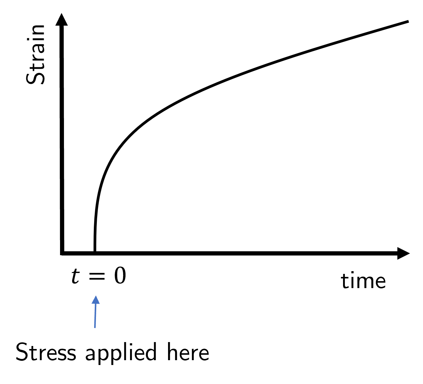
$A stress is applied at time $t=0$ and held constant. The strain $\gamma$ is observed as a function of time.$

Fig. 35 A stress is applied at time $t=0$ and held constant. The strain $\gamma$ is observed as a function of time.#

Stress relaxation modulus#

Similar to the creep compliance, we define the stress relaxation modulus $G(t)$ by considering an experiment in which a constant strain $\gamma_0$ is applied at time $t=0$, and this time the stress is measured as a function of time. Therefore the stress relaxation modulus is

\[\sigma(t) = \gamma_0G(t)\]

and the form of this function is shown in Fig. 36. The initial response is elastic, reaching a maximum $\propto G_0$, but decreases towards zero as the material starts to flow.

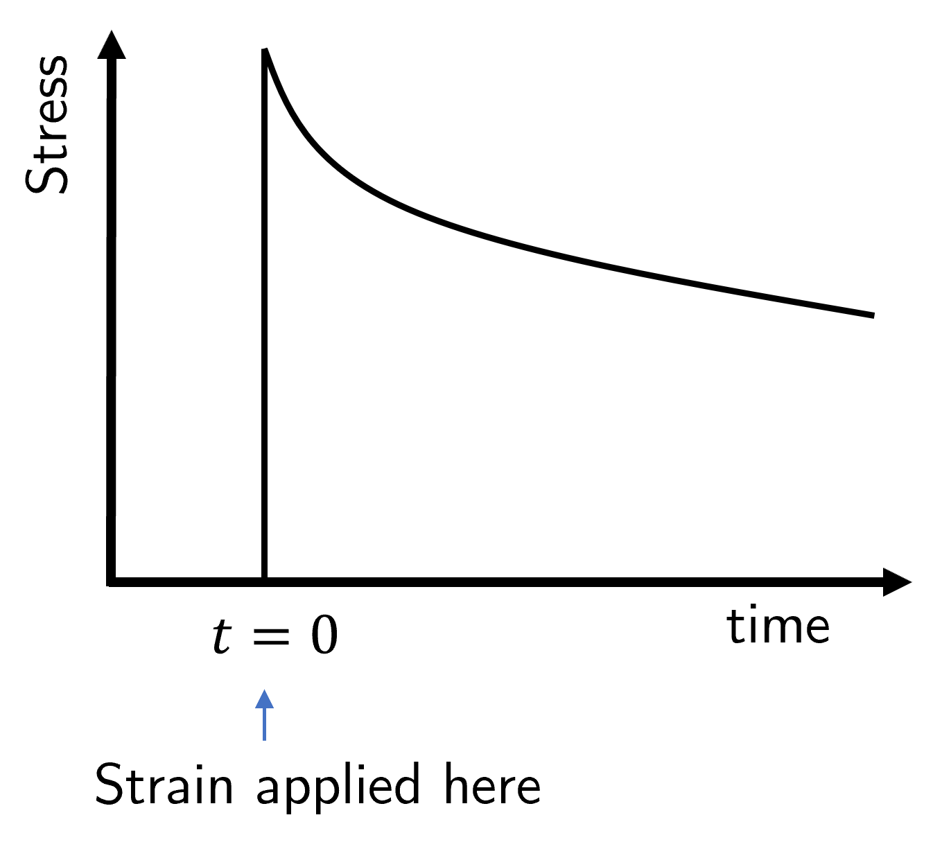
$A strain is applied at time $t=0$ and held constant. The stress $\sigma$ is observed as a function of time.$

Fig. 36 A strain is applied at time $t=0$ and held constant. The stress $\sigma$ is observed as a function of time.#

Characterising the viscoelastic behaviour.#

These conceptual experiments are a good place to start but at some point we will want to test this experimentally to see how well the model holds up in the real world. One of the earliest but still incredibly useful techniques is to apply an oscillatory deformation at a certain frequency $\omega$. This is useful experimentally as the equipment is not too challenging to build as shown in Fig. 37, but also the theoretical model is quite simple to understand.

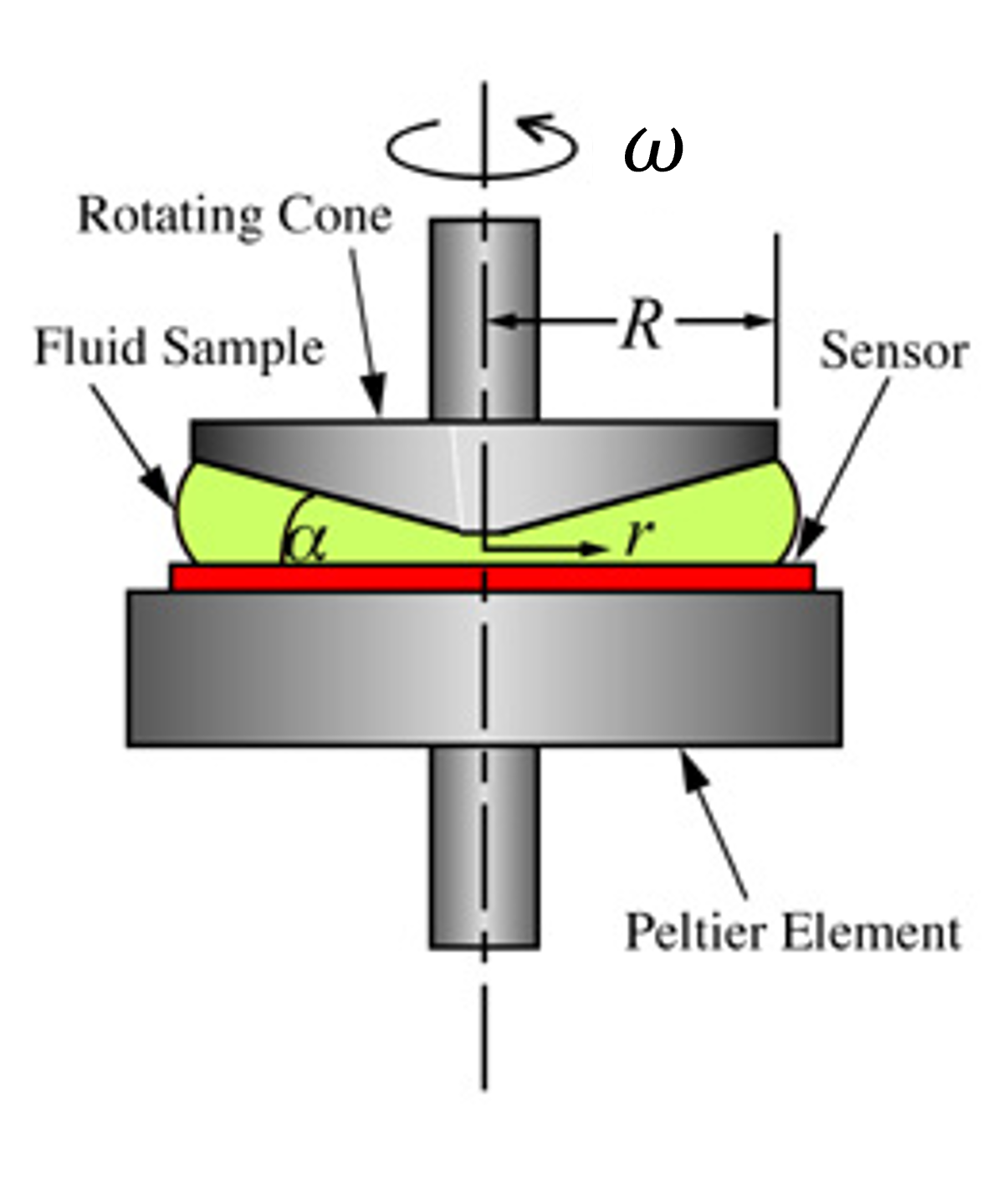
Fig. 37 A schematic of a cone and plate rheometer that applies an oscillatory strain to a sample.#

If the strain is oscillatory then it takes the form

\[\gamma(t) = \gamma_0\,\sin(\omega t)\]

If the material studied is a perfectly elastic solid then the stress in the sample will be related to the strain through Hookes’ law and so

\[\begin{split}\sigma(t) &= G_0\gamma(t)\\ &=G_0\gamma_0\sin(\omega t)\end{split}\]

The stress is perfectly in phase with the strain for a Hookean solid. On the other hand if the material being studied is a Newtonian liquid then the stress in the liquid will be related to the strain rate, i.e.

\[\begin{split}\sigma(t) = \eta\dot{\gamma} &= \eta\gamma_0\omega\cos(\omega t)\\ &= \eta\gamma_0\omega\sin\left(\omega t + \frac{\pi}{2}\right)\end{split}\]

The stress in a Newtonian liquid still oscillates with the same angular frequency $\omega$ but is out of phase with the strain by $\frac{\pi}{2}$.

You may wonder why I suddenly reverted back to considering these simple, non-viscoelastic materials. The reasoning is that the more interesting viscoelastic materials show both elastic and viscous behaviours so we can combine the Hookean and Newtonian cases to build our model for a viscoelastic material.

The critical observation here is that we can generalise the linear response of a viscoelastic material by introducing a general phase angle $\delta$ such that

\[\sigma(t) =G_0\gamma_0\sin(\omega t + \delta)\]

where $0\leq\delta\leq\frac{\pi}{2}$. Since the stress is always a sinusoidal function with the same frequency as the strain, we can separate the stress into two orthogonal functions that oscillate with the same frequency, one in phase with the strain and one $\frac{\pi}{2}$ out of phase with the strain,

\[\sigma(t) = \gamma_0\left[G'(\omega)\sin(\omega t)+G''(\omega)\cos(\omega t)\right]\]

where the complex modulus is $G^*(\omega) = G'(\omega)+G''(\omega)$. Here $G'(\omega)$ is the real part of $G^*(\omega)$ which corresponds to the storage modulus and relates to the elastic component of the response. The imaginary part, $G''(\omega)$ is the loss modulus and relates to the viscous component of the response.

Finally the complex modulus (a function in frequency) to the stress relaxation modulus (a function in time) are related by

\[G^*(\omega) = i\omega\int\limits_0^\infty \exp(-i\omega t)\,G(t)\,\mathrm{d}t\]

Time-temperature superposition - an experimental aside

We have seen that the viscoelastic responses of a material are a function of time, and experimental evidence shows that the viscoelastic properties of polymers are a strong function of temperature. A key discovery in this topic is that the relaxation times of all the modes have the same temperature dependence; this means it is possible to superimpose linear viscoelastic data taken at different temperatures, a process known as the time-temperature superposition principle. Stress relaxation modulus data taken at any given temperature $T$ can be superimposed on data at a reference temperature $T_0$ using a time scale muliplicative shift factor $\alpha_T$, such that

\[G(t,T) = G(\alpha_Tt,T_0)\]

and the temperature dependence of the shift factor has been found (empirically) to take the form

\[\log\alpha_T = \frac{-C_1(T-T_0)}{C_2+(T-T_0)}\]

where $C_1$ and $C_2$ are empirical constants. If we take the glass transition temperature as the reference emperature, i.e. $T_0 = T_g$ then we find that these two empirical constants have very similar values for many different polymers. If the logarithm in the previous equation is in base 10 then $C_1^g=17.4$ and $C_2^g=51.6\text{ K}$ are quasi-universal values. The superscript ‘g’ corresponds to ‘glass’ and emphasises the point that these values are true when the reference temperature is the glass transition temperature.

You might ask why this is a useful principle. In a perfect and hypothetical world we would be able to use our (perfect and hypothetical) experimental equipment to measure the module-time dependence across the entire range of time (or frequencies). In reality though our equipment is limited to a particular range of frequencies, and so this superposition principle allows us to shift our measured data into those lower or higher frequency ranges that our equipment cannot probe. We can use the data measured at some temperature $T$ and shift it onto a master curve for that particular polymer at a chosen reference temperature. An example of this is shown in Fig. 38.

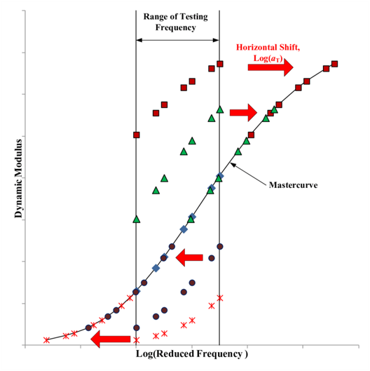
The dynamic modulus for a polymer is measured within a range of testing frequencies limited by the equipment used. The time-temperature superposition principle allows for these measured values to be shifted onto a master curve, where the dynamic modulus (as a function of frequency) is determined at a specific reference temperature.

Fig. 38 The dynamic modulus for a polymer is measured within a range of testing frequencies limited by the equipment used. The time-temperature superposition principle allows for these measured values to be shifted onto a master curve, where the dynamic modulus (as a function of frequency) is determined at a specific reference temperature.#

Viscoelasticity for polymer melts.#

Coming back to the matter at hand. If our simple materials have well defined phase shifts (zero for Hookean solid, $\frac{\pi}{2}$ for Newtonian fluid), then there must be some molecular explanation for why viscoelastic materials behave somewhere inbetween that explains the complex modulus behaviour we observe.

The way we study this is by experimentally measuring the relaxation modulus of different monodisperse polymer melts. Consider Fig. 39 in which two different monodispersions are depicted.

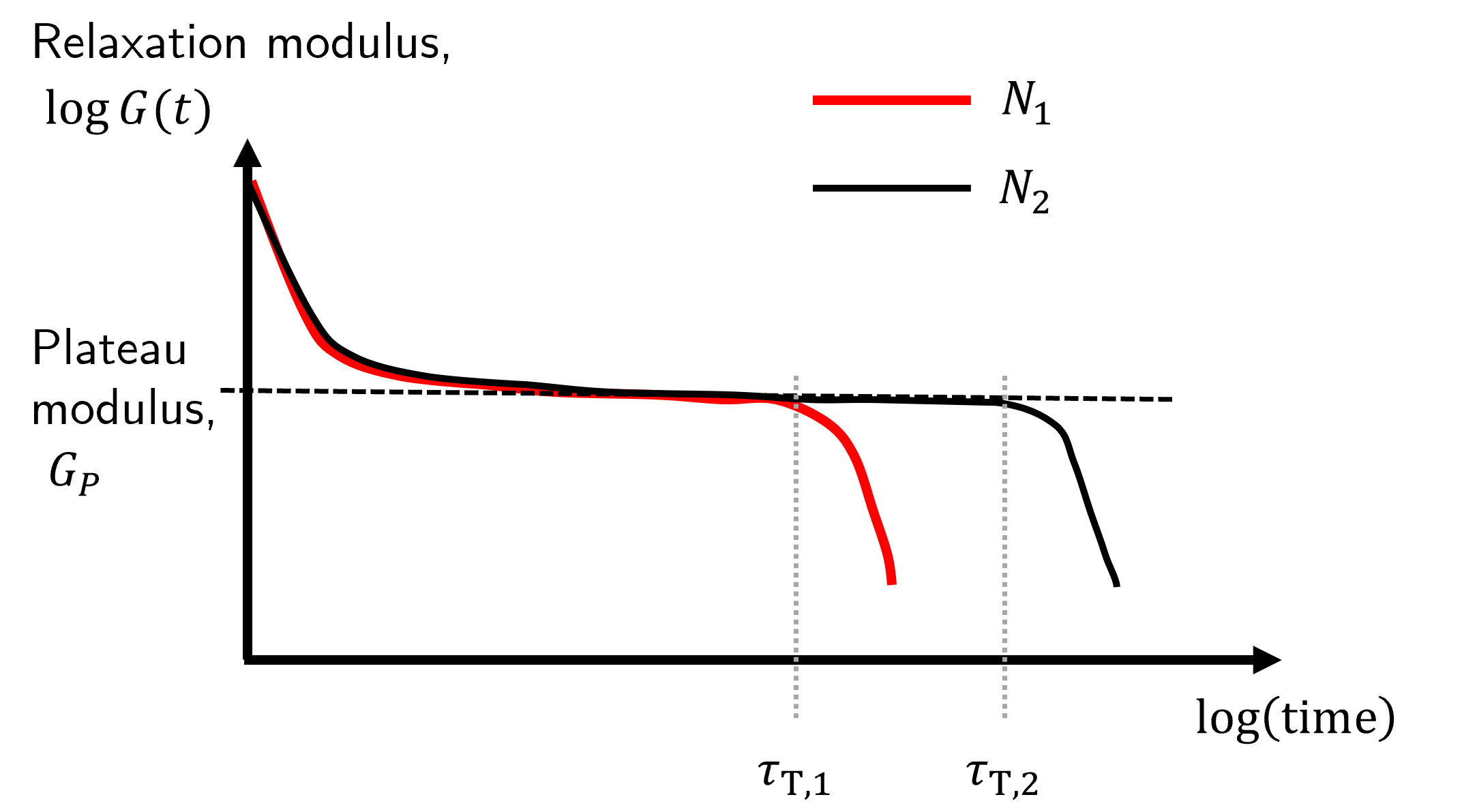
The relaxation curves are independent of $N$ in the initital relaxation (short time) and plateau (intermediate time) regions, but have a different terminal time in which the relaxation decreases again (longer timescales).

Fig. 39 The relaxation curves are independent of $N$ in the initital relaxation (short time) and plateau (intermediate time) regions, but have a different terminal time in which the relaxation decreases again (longer timescales).#

At short timescales the behaviour of the relaxation modulus is independent of $N$. At intermediate times the relaxation modulus is effectively constant at some plateau value, $G_P$, which is also independent of $N$. But at some longer characteristic timescale known as the terminal time, $\tau_\text{T}$, the relaxation modulus deviates from this plateau value. This terminal time does depend strongly on $N$ and is found to take the form $\tau_\text{T}\sim N^m$.

In the plateau region the polymer behaves like an elastic solid. After $\tau_\text{T}$ the polymer flows in a viscous-like manner and the creep compliance varies as $J(t)\sim t$. The zero shear viscosity, $\eta_0$, i.e. the viscosity a polymer melt would have in the absence of an external shear is related to both the terminal time and plateau modulus as

\[\eta_0 \sim \tau_\text{T}G_P\]

Noting again that because the plateau modulus is independent of $N$, any relationship between zero shear viscosity and $N$ should be the same as that between terminal time and $N$. Thus

\[\eta_0 \sim N^m\]

Experimental data tells us that $m\approx3.4$, but only above some certain critical value $N_C$. Below this the relationship between $\eta_0$ and $N$ is linear, i.e.

\[\begin{align*} \eta_0 \sim \begin{cases} N &\text{if $N<N_C$}\\ N^{3.4} & \text{if $N>N_C$} \end{cases} \end{align*}\]

If you don’t believe me then take a look at the first experimental evidence of this on the polymer polybutediene [Colby et al., 1987], and the relevant figure from this paper is shown in Fig. 40.

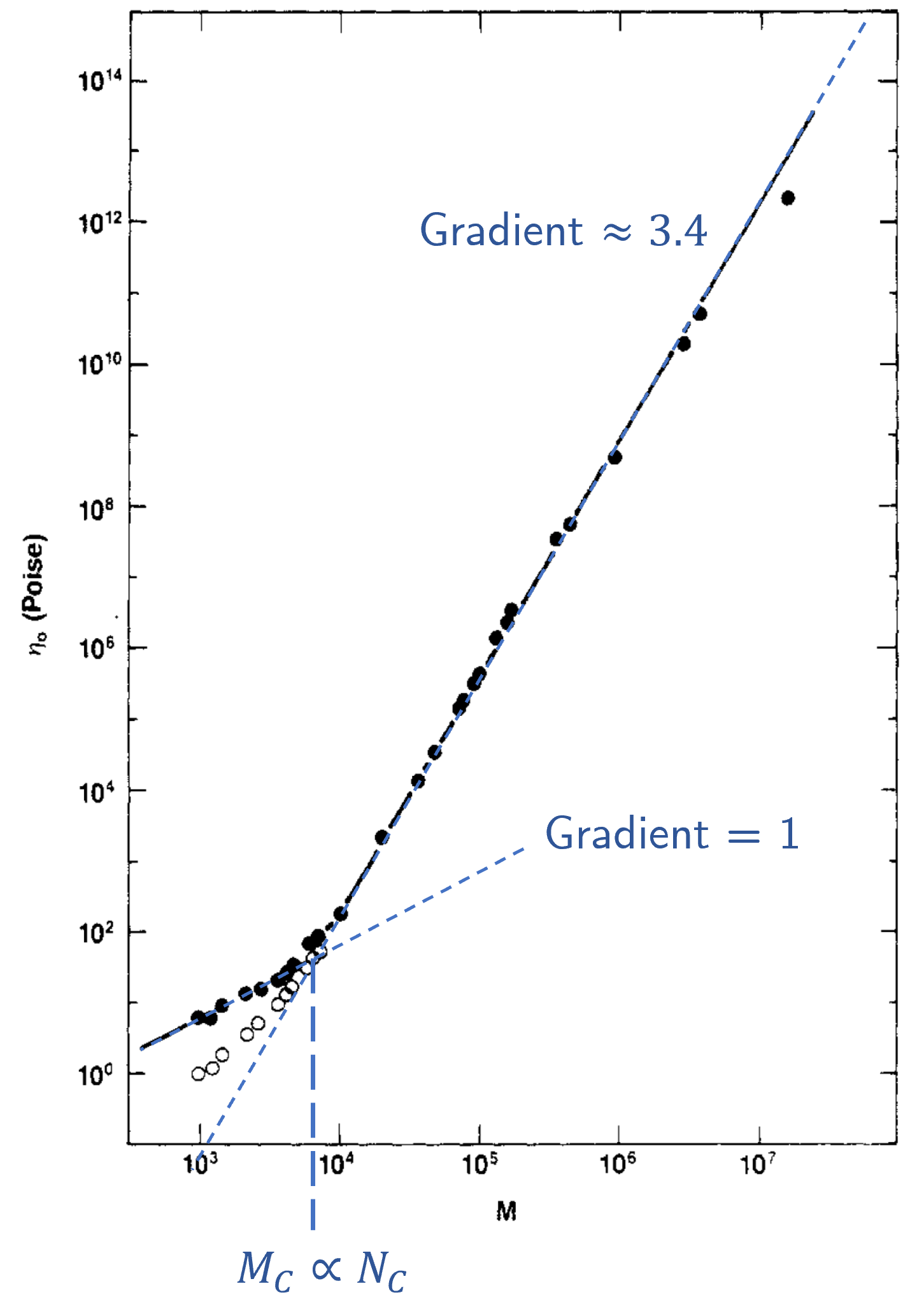
Zero shear velocity measured for different relative molecular masses (which depends on $N$) of polybutadiene. Dashed lines in blue have been added by me to show the two different behaviours below and above $N_C$. The critical molecular mass $M_C$ is indicated here, but this is proportional to $N_C$.

Fig. 40 Zero shear velocity measured for different relative molecular masses (which depends on $N$) of polybutadiene. Dashed lines in blue have been added by me to show the two different behaviours below and above $N_C$. The critical molecular mass $M_C$ is indicated here, but this is proportional to $N_C$.#

Let us pull together a lot of the different topics we’ve covered so far. This last section tells us that the viscosity of a viscoelastic material depends on the number of units in a chain, $N$. We have previous seen that the size of a polymer chain also depends on $N$. Finally we also saw that the charactistic timescales in which particles can ‘escape’ from a ‘cage’ depends on the size of the molecule (through the interaction between it and surrounding molecules).

This leads us to a nice point of convergence: can we understand why viscoelastic materials behave they way they do if we understand how long chain molecules of a characteristic size can move when also interacting with neighbouring molecules? The answer lies in how polymer chains in the melt are entangled, which (with a little thought) could come out from the data in Fig. 40; short chain polymers behave more like small colloidal particles, but once the chains get to a certain length they are able to intertwine and entangle. An alternative view is that it is unlikely that a bunch of really short lengths of string mixed in a container will form a tangled mess, but this is very likely for long lengths of string.

Entanglement and reptation.#

If our polymers are long, linear objects which cannot pass through one another, then we can imagine that a polymer melt is a mess of long and extended in some random network of interpenetrating chains. If we apply a shear to this network of chains then they will become more tangled up which would then make it harder to shear the material any further.

With this conceptual model in mind we can imagine the rubber-like plateau modulus arising from the entanglements between chains acting as temporary physical crosslinks. As the plateau modulus is independent of $N$ we can estimate the density of entanglements or the average distance between entanglement points. We can modify equation (37) as

\[G = \frac{\rho R T}{M_e}\]

where $M_e$ is the average relative molecular mass between entanglements. These entanglements are not permanent and can disentangle with a characteristic timescale comparable to the terminal time $\tau_\text{T}$. Intuitively we expect shorter chains (smaller $N$) to require less time to disentangle, but can we formalise this more to see whether the concept of entanglement can predict the $\tau_\text{T}\sim N^{3.4}$ behaviour seen previously.
The short answer is yes, sort of. We will consider one of the initial models proposed that does go some part of the way, known as the tube model of reptation.

Tube model and reptation#

Let us consider the behaviour of a single chain amongst all others in the melt. These other chains act as fixed barriers that our single chain of interest cannot pass, and so we can represent these other chains as points in space. Consequently there exists a tube volume around our single chain in which it can move around. This is shown schematically in Fig. 41 where for simplicity we align our single chain in the plane of the page and have the fixed chains aligned perpendicular to the page. Crosses show the position of where these fixed chains intersect the plane.

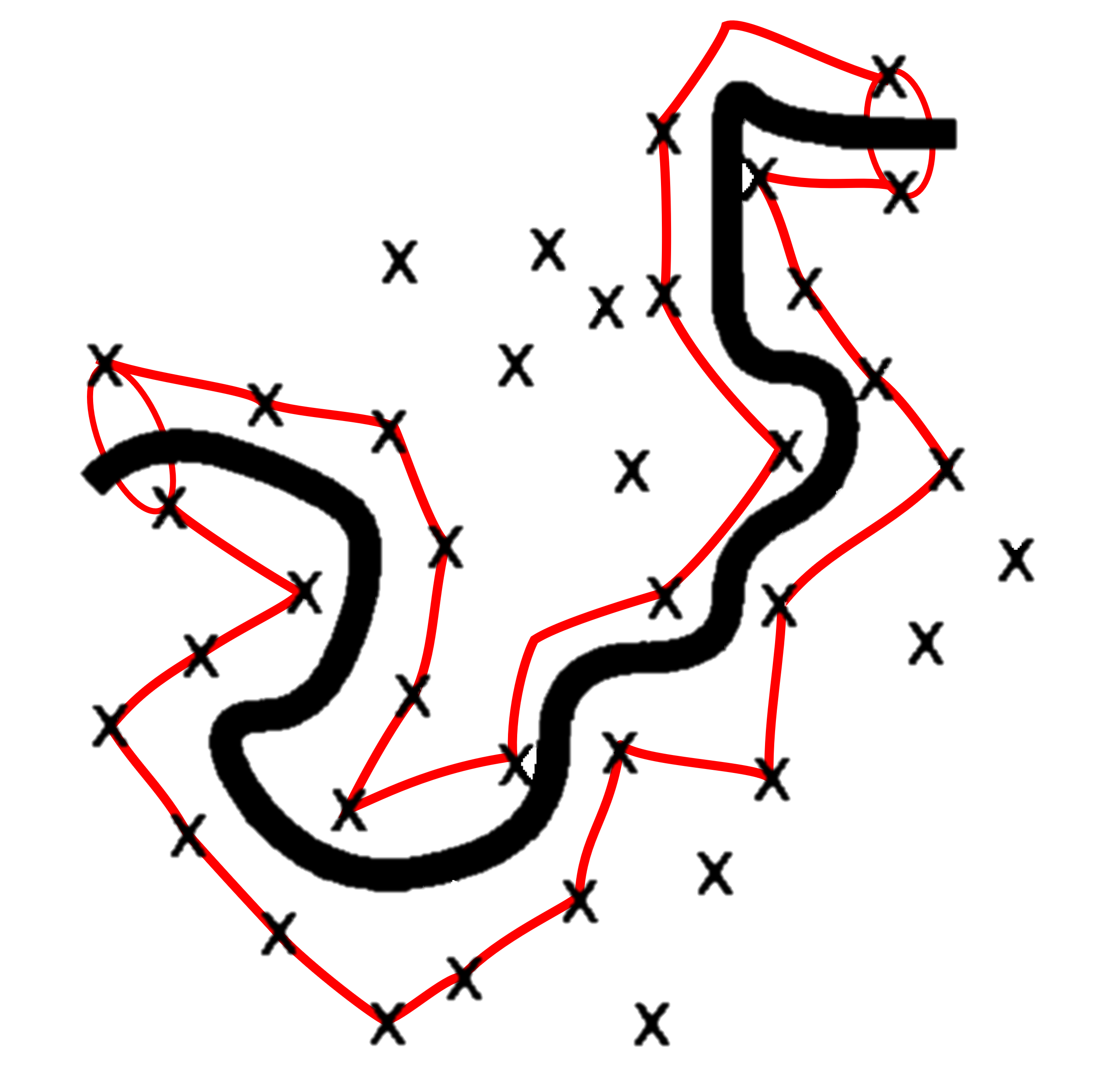
The tube model of a polymer melt. The single chain of interest (black line) is found in the plane of the page, and the other fixed chains point into / out of the page, indicated by crosses. The red tube encloses the volume in which our single chain can move without 'hitting' a fixed chain.

Fig. 41 The tube model of a polymer melt. The single chain of interest (black line) is found in the plane of the page, and the other fixed chains point into / out of the page, indicated by crosses. The red tube encloses the volume in which our single chain can move without ‘hitting’ a fixed chain.#

We can now determine the characteristic time that it would take for this single polymer chain to wiggle its way out of the chain. This type of motion is known as reptation and is indeed a wiggle much in the same way that a snake moves. The difference is that a snake moves in a well choreographed way whereas our polymer chain will be moving under random walk statistics with the constraint that a step cannot cause any part of the single chain to pass through a fixed chain.

Deriving the Stokes-Einstein model for a single particle.

Important: This dropdown section is included for completeness but falls outside of the core curriculum for this module. Understanding it will help reinforce your knowledge of random walk systems, but the derivation itself is not examinable

I am making an assumption that you are familiar with the history and concept of Brownian motion, so will just start from the idea that a particle undergoing Brownian motion is displaying a random walk type of motion. We see that the particle is changing position at successive small intervals of time but these position changes are not correlated - the direction of the $n^\text{th}$ step is not influenced by the direction of the $(n-1)^\text{th}$ step.

Because the direction of each step is random we expect the time average of the displacement vector $\textbf{R}(t)$ to be zero, however the mean value of the square of the displacement will be proportional to the time we have observed the particle for (i.e. the number of steps the particle has taken). We can formalise this as

(38)#\[\begin{align} \left<\left(\textbf{R}(t)\right)^2\right>&= \zeta t \end{align}\]

where the constant of proportionality $\zeta$ the drag coefficient and relates to the resistance of motion through a fluid.

So what is the net force acting on our particle? You have already seen this as part of your first year mechanics course but I’ll be nice and give a bit of a reminder! We assume that the drag force on a particle moving through a fluid is proportional to the velocity - in my first year notes I used $F_\text{drag}=bv$ but now we use $F_\text{drag}=\zeta v$. This is nothing more than a symbol change.

Thus the net force on a particle undergoing random motion is

(39)#\[F_\text{random} = m\frac{\mathrm{d}^2\textbf{R}}{\mathrm{d}t^2}+\zeta\frac{\mathrm{d}\textbf{R}}{\mathrm{d}t}\]

Before moving on I’ll emphasise the difference between this and what you saw in the first year mechanics. The mechanics case was a body falling vertically under gravity but also through a resistive medium, which is why the first year notes include an $mg$ term. In this Brownian motion case we are dealing with a system in which the particles are small enough such that the effect of gravity is significantly small compared to the forces and interactions causing the Brownian motion.

This different allows us to make a generalisation about the displacement vector. If gravity is not a signficiant factor in the system then there is no difference in the way the particle behaves in the $x$, $y$ and $z$ directions. Thus

\[\begin{split}\left<x^2\right> &= \left<y^2\right> = \left<z^2\right>\\ \therefore \left<\textbf{R}^2\right> &= \left<x^2\right>+\left<y^2\right>+\left<z^2\right>\\ &= 3\left<x^2\right>\end{split}\]

which allows us to rewrite equation (39) as

(40)#\[\begin{split}F_\text{random} &= 3m\frac{\mathrm{d}^2(x^2)}{\mathrm{d}t^2}+3\zeta\frac{\mathrm{d}(x^2)}{\mathrm{d}t}\\ \zeta\frac{\mathrm{d}(x^2)}{\mathrm{d}t} &= \frac{F_\text{random}}{3} - m\frac{\mathrm{d}^2(x^2)}{\mathrm{d}t^2}\end{split}\]

Take care here. We need to remember that $x$ is a function of $t$, so we need to simplify the differential terms using the chain and product rules, i.e.

\[\begin{split}\frac{\mathrm{d}(x^2)}{\mathrm{d}t} &= \frac{\mathrm{d}x^2}{\mathrm{d}x}\frac{\mathrm{d}x}{\mathrm{d}t} = 2x\frac{\mathrm{d}x}{\mathrm{d}t}\\ \frac{\mathrm{d}^2(x^2)}{\mathrm{d}t^2} &= 2\left(\frac{\mathrm{d}x}{\mathrm{d}t}\right)^2 + 2\frac{\mathrm{d}}{\mathrm{d}t}\left(x\frac{\mathrm{d}x}{\mathrm{d}t}\right)\end{split}\]

Chuck all of these into equation (40) and take the time average of each term to get

(41)#\[\frac{\zeta}{2} \frac{\mathrm{d}\left<x^2\right>}{\mathrm{d}t} = \frac{\left<F_\text{random}\right>}{6} - m\left<\left(\frac{\mathrm{d}x}{\mathrm{d}t}\right)\right>^2 - m \frac{\mathrm{d}}{\mathrm{d}t}\left<x\frac{\mathrm{d}x}{\mathrm{d}t}\right>\]

We can make some simplifications here based on the time average. As there is no directional preference of the force we expect the average force to be zero. Similarly there is no correlation between the position and velocity of the particle, so the right hand term of equation (41) is also zero. The remaining middle term is simply twice the kinetic energy, and we can thus drop the minus sign in front. The kinetic energy associated with our Brownian particle comes from the thermal energy of the system at temperature $T$, which gives

\[\begin{split}\frac{\mathrm{d}\left<x^2\right>}{\mathrm{d}t} &= 2\frac{k_\text{B}T}{\zeta}\\ \therefore \left<\textbf{R}^2\right> &= \frac{6k_\text{B}T}{\zeta}t = 6Dt\end{split}\]

where

(42)#\[D=\dfrac{k_\text{B}T}{\zeta}=k_\text{B}T\mu\]

$D$ is the diffusion coefficient that was derived by Einstein in his seminal work on Brownian motion and $\mu$ is the mobility of the particle (defined as $\mu=\frac{1}\zeta$).

Without going into the details around the derivation, Stokes’ theorem allows us to define the drag coefficient in terms of the viscosity of the surrounding medium $\eta$ and the radius of the diffusing particle $a$, namely

(43)#\[\zeta = 6\pi\eta a\label{eq:C1_StokesEq}\]

and so we finally can show that the diffusion coefficient (a measure of mobility of single particles) is

(44)#\[D_\text{SE} = \frac{k_\text{B}T}{6\pi \eta a}\label{eq:C1_StokesEinstein}\]

The key equation we need going forward from the Stokes-Einstein derivation is (42), i.e. $D=k_\text{B}T\mu$.

In the dropdown box above we considered the Brownian motion of a single particle ($N=1$) but for our polymer chain we have $N$ segments forming the chain. Thus if we define the mobility of an individual segment as $\mu_\text{seg}$ then the total mobility of the tube is

\[\mu_\text{tube} = \frac{\mu_\text{seg}}{N}\]

where we have assumed that the viscous force of the whole chain is the sum of the forces experienced by the individual segments. Plugging this into the Einstein relation above gives.

\[\begin{split}D_\text{tube} &= k_\text{B}T\mu_\text{tube}\\ &= \frac{k_\text{B}T\mu_\text{seg}}{N}\end{split}\]

Our single chain is essentially undergoing a one dimensional random walk within the tube. If the tube length is $L$ then the time taken for the polymer to random walk this length is

\[\begin{split}\tau_\text{T} &= \frac{L^2}{D_\text{tube}}\\ &= \frac{NL^2}{k_\text{B}T\mu_\text{seg}}\end{split}\]

As the chain is extended we expect the length of the tube to be proportional to the number of units in the chain, meaning

\[\begin{split}\tau_\text{T} &\sim NN^2\\ &\sim N^3\end{split}\]

So this simple tube model predicts $\tau_\text{T} \sim N^3$ compared to the $\tau_\text{T}\sim N^{3.4}$ found experimentally. This is not too bad but refinements to the model allow us to get closer to the experimentally determined value. Two of these changes are

Constraint release, in which we recognise that the originally fixed chains (crosses in figure \label{fig:C2_Rep} are themselves single chains moving in their own tubes, and
Contour length fluctuations, in which the length of the tube is assumed to be linear with $N$ the fluctuationing, $a\sqrt{N}$ end-to-end distance is more appropriate for the tube length.

These are included here for you to think about but the detail is beyond the scope of the course.

Polymer gels and polymer brushes.#

Before we finish this section I wanted to consider two different types of polymer systems that I think are pretty cool but, probably more importantly, have some wider applicability in materials science and biophysics. Both of these systems arise when we somehow permanently bond the polymer chains to something, either to each other to form a gel or to a surface to form a polymer brush.

Polymer gels}#

Consider the case in which the chains in a polymer melt are entangled, and these entanglements are sufficiently long lived that they act as (semi) permanent crosslinks. If this network of polymer chains is swollen in a solvent, such that solvent molecules try to permeate the network and cause it to expand, then the resulting material is known as a gel[^C2_Sol-Gel]. The gel effectively becomes a single, almost infinite hyperbranched polymer.

The volume fraction $\phi$ of a swollen polymer gel is the ratio of the swollen and dried state volumes, $V$ and $V_\text{dry}$, namely

\[\phi = \frac{V}{V_\text{dry}}\]

Note that $V$ is the total volume of the polymer and of the solvent within the gel.

Let $\phi_0$ be the polymer volume fraction in the preparation state when the crosslinking was performed (i.e. when we made the gel) with an associated gel volume $V_0$. Assuming that the gel is well developed (and not a sol-gel2) then the total amount of polymer in the gel does not change when the gel is swollen or deswollen. Under this assumption the change in volume when swelling is due entirely to the change in the amount of solvent in the gel, meaning

\[V_0\phi_0 = V\phi = V_\text{dry}\]

We now make use of the affine deformation assumption such that an unconstrained network polymer with swell uniformly by the same amount in each direction. Thus the linear deformation $\lambda$ is simply

\[\lambda = \left(\frac{V}{V_0}\right)^{\frac{1}{3}} = \left(\frac{\phi_0}{\phi}\right)^{\frac{1}{3}}\]

When the network is swollen each network strand is stretched as the crosslink junctions move further apart. Recalling the free energy required to stretch an ideal chain (see equation (29)) we can state that the free energy associated with this affine deformation is

(45)#\[F_\text{el} \approx k_\text{B}T\frac{\left(\lambda R_0\right)^2}{Na^2}\]

or

(46)#\[F_\text{el} \approx k_\text{B}T\frac{\left(\lambda R_0\right)^2}{R_\text{Ref}^2}\label{eq:C2_Panyukov}\]

Equation (46) is known as the Panyukov form and considers the elastic energy of a swollen network strand in terms of $R_\text{Ref}^2$, the mean-square fluctuations of the end-to-end distance of the network strand. In many cases $R_\text{Ref}^2$ is equal to the mean-squared end-to-end distance of a free chain with the same $N$ as the network strand3.

As the network swells, either because more solvent is permeating the network or because the quality of the solvent changes, the strand elasticity changes because $R_\text{Ref}^2$ changes.
The modulus of the gel in the swollen state, $G(\phi)$ is proportional to the chain number density $\nu=\dfrac{\phi}{Na^3}$ times the elastic free energy per chain given above, so

(47)#\[\begin{split} G(\phi) &\approx \nu k_\text{B}T\frac{\left(\lambda R_0\right)^2}{R_\text{Ref}^2}\\ &\approx \frac{k_\text{B}T}{a^3}\frac{\phi}{N}\frac{\left(\lambda R_0\right)^2}{R_\text{Ref}^2}\end{split}\]

At the swelling equilibrium the elasticity is balanced by the osmotic pressure $\Pi$ of a semidilute solution of uncrosslinked chains at the same concentration. We’ve already seen that the modulus is proportional to the elastic free energy (per unit volume) which means the gel will swell until the modulus and osmotic pressure are balanced.

At this equilibrium point we can define the swelling ratio $Q$ in terms of the equilibrium volume $V_\text{eq}$ and the dried state volume $V_\text{dry}$:

(48)#\[Q = \frac{V_\text{eq}}{V_\text{dry}} \qquad\qquad \text{when $G\approx\Pi$}\]

This may seem like a rather flippant and irrelevant definition but it gives us a good link between the experimental (macroscopic) domain and quantifying the molecular structure. We will only consider a particular special case but if you are interested there is a more comprehensive coverage in Polymer Physics by Rubinstein and Colby [Rubinstein, 2003].

Swelling a gel in $\theta$-solvents}#

Firstly, a definition. A $\theta$-solvent is the solvent in a polymer-solvent pair for which there exists a $\Theta$ temperature.
By definition, the mean-squared end-to-end distance of a free chain in a $\theta$-solvent is independent of concentration, with $R_0^2\approx a^2N$. The fluctuations of a network strand that control its elasticity are also independent of concentration, so

\[R_\text{ref}^2\approx R_0^2 \approx a^2N\]

Hence the more general Panyukov form (equation (46)) reduces to the Flory form (equation (45)) for swelling in $\theta$-solvents.
Substituting this into equation (47) gives us the gel modulus in a $\theta$-solvent

(49)#\[\begin{split}G(\phi) &\approx \frac{k_\text{B}T}{a^3}\frac{\phi}{N}\lambda^2\\ &\approx \frac{k_\text{B}T}{Na^3}\phi_0^\frac{2}{3}\phi^\frac{1}{3}\end{split}\]

I will now introduce without proof4 a definition for the osmotic pressure of a semidilute solution in a $\theta$-solvent, namely

(50)#\[\Pi \approx \frac{k_\text{B}T}{a^3}\phi^3\label{eq:C2_Osmotic}\]

We can combine this equation with equations (48) and (49) gives

\[Q\approx \frac{N^\frac{3}{8}}{\phi_0^\frac{1}{4}}\]

and if the network was prepared in the dry, solvent-free state such that $\phi_0=1$ then we find that

\[N \approx Q^\frac{8}{3}\]

Pause and reflect on what this is telling us. When working with a network in a $\theta$-solvent we can determine the average number of monomers in a network strand by simply weighing a piece of gel when it is dry and again after it has reached an equilibrium swelling volume. These two measurements are so incredibly easy to do that we could do it using the weighing scales in the teaching lab, whereas determining $N$ directly (using neutron scattering, x-ray scattering, FCS, etc…) requires very sophisticated equipment and analysis.

Polymer brushes#

Let us now conclude this section by considering polymers interacting with a surface. There are two cases that we could consider (shown in Fig. 42) where either the polymers are adsorbed onto the surface through relatively weak interactions or one end of the polymer chains is strongly tethered to the surface.

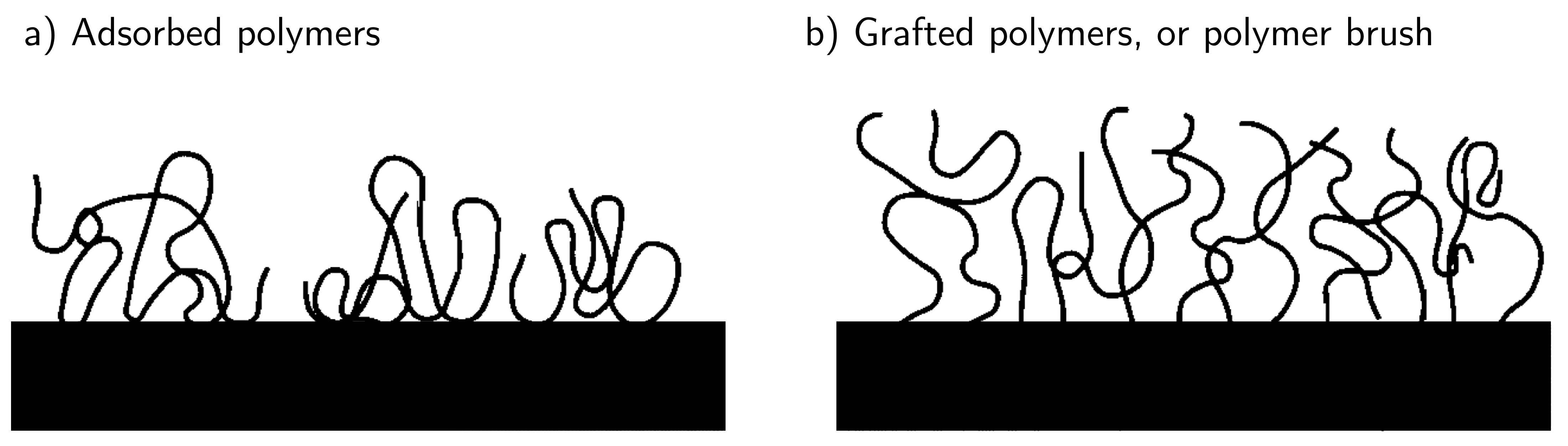
Polymer chains are either laying on the surface with random monomer units interacting with the surface or are affixed at one end to a horizontal surface and the free ends are dangling upwards into the solvent.

Fig. 42 Polymer chains are either laying on the surface with random monomer units interacting with the surface (adsorbed) or are affixed at one end to a horizontal surface and the free ends are dangling upwards into the solvent (polymer brush).#

We will skip the former because that topic in itself is a whole module, but the tethered molecules case is much simpler to model.

We will consider the case in which the molecules are relatively densely packed in terms of their grafting density.\footnote{The other extreme is isolated chains that have no interaction with other tethered chains. This is less interesting because they tend to follow non-ideal chain statistics, i.e. $\left<R^2\right>\sim N^\frac{3}{5}$.} If we define this grafting density as $\dfrac{\sigma}{a^2}$ chains per unit area and note that the volume per chain is $\dfrac{ha^2}{\sigma}$ then the total energy is

\[F_\text{Total} = F_\text{el}+F_\text{rep}+U_\text{int}\]

where $F_\text{el}$ is the free energy of stretching like an elastic chain, i.e.

\[F_\text{el} = k_\text{B}T\frac{h^2}{Na^2}\]

and $F_\text{rep}+U_\text{int}$ are the combined excluded volume and interaction energies

\[F_\text{rep}+U_\text{int} = k_\text{B}Tb(1-2\chi)\frac{\sigma N^2}{2ha^2}\]

where $b$ corresponds to the finite volume of a polymer of $N$ units collapsed into a sphere. Thus

\[\begin{split}F_\text{Total} &= k_\text{B}T\frac{h^2}{Na^2} + k_\text{B}Tb(1-2\chi)\frac{\sigma N^2}{2ha^2}\\ &= \frac{k_\text{B}T}{a^2} \left[ \frac{h^2}{N} + b(1-2\chi)\frac{\sigma N^2}{2h}\right]\end{split}\]

Minimising this free energy with respect to brush height (i.e. when $\dfrac{\mathrm{d}F}{\mathrm{d}h}=0$) allows us to find the equilibrium brush height of

\[h \sim \left[\sigma b(1-2\chi)\right]^\frac{1}{3}N\]

This tells us that chains grafted to a surface at a sufficiently high density will overlap significantly and the result is that the chains are strongly stretched to approximately a straight chain where $h\sim N$.

1: The core textbook by Jones uses $\tau$ for tensile stress. I prefer not to because $\tau$ to me is a time constant, and one that we’ve used heavily in this chapter already.}
2: Textbooks may refer to a sol-gel. This is the general form that recognises some of the polymer chains (the sol) may not be attached to the gel. Given that this is a brief introduction we will assume that all of the polymer chains form part of the network.
3: The size the network strand (i.e. polymer chain) would have if it were detached from the network and put into a vacuum or solvent, depending on which model you use.
4: Section 5.4.2 of [Rubinstein, 2003] if interested but it is not required for this course.

Bibliography

- CFG87
Ralph H. Colby, Lewis J. Fetters, and William W. Graessley. The melt viscosity-molecular weight relationship for linear polymers. Macromolecules, 20(9):2226–2237, 1987. URL: https://doi.org/10.1021/ma00175a030, arXiv:https://doi.org/10.1021/ma00175a030, doi:10.1021/ma00175a030.
- Rub03(1,2)
Michael Rubinstein. Polymer physics. Oxford University Press, Oxford ; New York, N.Y., 2003. ISBN 9780198520597.