2.2 Polymers: Ideal Chain

2.2 Polymers: Ideal Chain#

Size of ideal chain#

In this model we assume that our polymer chain is made up of \(N\) units of individual length \(a\). If we then attach a vector \(\textbf{a}_i\) to each unit pointing to the next (i.e. pointing from unit \(i\) to \(i+1\)) unit then we are describing our polymer as a random walk in space. There is an important assumption here in that the orientation of each unit is random and independent of the direction of any other unit. An odd outcome of this is that it is possible for units of the chain to occupy the same space. This is why it is called an ideal chain, and we will address partly by considering the effect of short-range interactions and then in more depth when we consider what are termed real chains.

We shall consider simplest possible model where we assume that the chain follows a regular lattice. In the two dimensional case shown in Fig. 24 each vector has 4 possible directions (up, right, left, and down), and moves a single step in any of these direction. This step is denoted \(\textbf{a}_i\) and the size is equal to one lattice spacing.

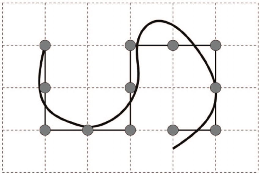
We can model a polymer chain (black) as a two-dimensional lattice where the ends of the segments are circles and as such the segments themselves lie only on the lattice lines.

Fig. 24 We can model a polymer chain (black) as a two-dimensional lattice where the ends of the segments are circles and as such the segments themselves lie only on the lattice lines.#

The end-to-end vector \(\textbf{r}\) is thus the sum of the individual vectors \(\textbf{a}_i\). The average value of the end-to-end vector, \(\left<\textbf{r}\right>\) is zero - the random directions each vector can take means it is equally likely for it to point along opposing directions1. However the average square of the end-to-end vector, \(\left<\textbf{r}^2\right>\) will tell us what we want to know. We need to take the average of all possible products between individual vectors, as follows:

(16)#\[\begin{split}\left<\textbf{r}^2\right> &= \left<\left(\sum\limits_{i=1}^{N}\textbf{a}_i\right)\cdot\left(\sum\limits_{j=1}^{N}\textbf{a}_j\right)\right>\\ &= \left<\sum\limits_{i=1}^{N}\sum\limits_{j=1}^{N}\textbf{a}_i\cdot\textbf{a}_j\right>\\ &= Na^2 + \left<\sum\limits_{i\neq j}\textbf{a}_i\cdot\textbf{a}_j\right> \label{eq:C2_Ideal1}\end{split}\]

where I have taken out the \(N\) cases for \(i=j\) which makes the dot product simply equal to \(a^2\). The right hand side of equation (16) is easy to evaluate when we remember that the direction of one vector is independent and not correlated with any other vector. This means that the dot product for \(i\neq j\) vectors averages to zero. Thus we can state that the average (that is, the root-mean-square) size of our polymer is

(17)#\[\sqrt{\left<\textbf{r}^2\right>} = aN^\frac{1}{2}\label{eq:C2_Ideal2}\]

The take home prediction is that the average size of our is proportional to the distance between units and the square root of the number of units in the chain. It turns out that this rather simple approximation is extremely good, more so than we would expect from the rather simple and constrained assumptions made.

Probability distribution of an ideal chain#

Now that we have some model for the average end-to-end distance, it is insightful to also calculate the probability distribution of \(\textbf{r}\) to get some feel for the spread of possible \(\textbf{r}\) values.
First we assume that one end of our chain of \(N\) bonds is fixed at the origin. Let \(P(\textbf{r}, N)\) be the probability that the other end of the polymer is at position \(\textbf{r}\). If we state that \(\textbf{a}_{i=1,\ldots,z}\) are the possible bond vectors the polymer can take, we can see that if the polymer has position \(\textbf{r}\) and \(N\) steps then the position vector at the \((N-1)^\text{th}\) step must take one of the possible \(\textbf{r}-\textbf{a}_i\). There are \(z\) possibilities here so, assuming each are equally likely, each has a probability of \(\frac{1}{z}\) of occuring. Thus the probability of the polymer end being at \(\textbf{r}\) can be written as

\[P(\textbf{r},N) = \frac{1}{z}\sum\limits_{i=1}^zP(\textbf{r}-\textbf{a}_i,N-1)\]

Assuming the polymer is very long, such that \(N\gg1\) and \(\left|\textbf{r}\right|\gg\left|\textbf{a}_i\right|\) then the right hand side can be expanded as

\[P(\textbf{r}-\textbf{a}_i,N-1) = P(\textbf{r},N) - \frac{\partial P}{\partial N}-\frac{\partial P}{\partial r_\alpha}a_{i\alpha}+\frac{1}{2}\frac{\partial^2P}{\partial r_\alpha \partial r_\beta}a_{i\alpha}a_{i\beta}\]

where \(a_{i\alpha}\) and \(R_\alpha\) are components of \(\textbf{a}_i\) and \(\textbf{r}\), and I have used the Einstein convention for summation over repeated indicies. We next use this expansion in the previous equation and simply using

(18)#\[\begin{align} \frac{1}{z}\sum\limits_{i=1}^za_{i\alpha}&=0 & \frac{1}{z}\sum\limits_{i=1}^za_{i\alpha}a_{i\beta}=\frac{\delta_{\alpha\beta}a^2}{3} \end{align}\]

means that

(19)#\[\frac{\partial P}{\partial N} = \frac{a^2}{6}\frac{\partial^2 P}{\partial \textbf{r}^2}\]

Equation (19) is a differential equation that can be solved using the condition that \(\textbf{r}=0\) when \(N=0\) (i.e. \(\textbf{r}\) is at the origin when \(N=0\) or at the start of the chain), which gives

(20)#\[P(\textbf{r},N) = \left(\frac{3}{2\pi Na^2}\right)^{\frac{3}{2}}\,\exp\left(-\frac{3\textbf{r}^2}{2Na^2}\right)\]

Effect of short-range interactions#

I previously mentioned the slightly unusual situation where our simple ideal chain model allows for units to occupy the same space. Or rather we have not introduced any constraints that prevent this obviously unphysical situation from occuring. We shall now address this issue in part - the most substantial approach will be covered when we look at the Real chain.

Let us only consider the effect of short-range interactions. It is possible for us to introduce some constraint on adjacent units, and ensure that the bond vector \(\textbf{r}_{n+1}\) is not allowed to point back to the previous step / unit. In other works we impose the restriction that \(\textbf{r}_{n+1}\neq-\textbf{r}_n\). Instead the \((n+1)\) vector must take one of the remaining \((z-1)\) directions at random. Thus the average value of \(\textbf{r}_{n+1}\) will not be zero for a given \(\textbf{r}_{n}\) because it can point along \(\textbf{r}_{n}\) but not \(-\textbf{r}_{n}\), creating an asymmetry in the possible configuration space.
We can still make use of the fact that the sum of all possible vectors is zero but modify it slightly to include the constraint previously mentioned, i.e.

\[\begin{split}0 &= \sum\limits_{i=1}^z\textbf{a}_i\\ &= (z-1)\left<\textbf{r}_{n+1}\right>_{\textbf{r}_n}-\textbf{r}_n\\ \therefore \left<\textbf{r}_{n+1}\right>_{\textbf{r}_n} &= \frac{1}{z-1}\textbf{r}_n\end{split}\]

from which we then find that

\[\left<\textbf{r}_{n+1}\cdot\textbf{r}_n\right> = \frac{a^2}{z-1}\]

That sorts out a relationship between adjacent chains, but what about the effect between the \(n\) and \((n+2)\) chain? For this we want to calculate \(\left<\textbf{r}_{n+2}\cdot\textbf{r}_n\right>\) for a fixed \(\textbf{r}_{n+1}\) which is found by

\[\begin{split}\left<\textbf{r}_{n+2}\cdot\textbf{r}_n\right> &= \left<\left<\textbf{r}_{n+2}\right>_{\textbf{r}_{n+1}}\cdot\textbf{r}_n\right>\\ &= \frac{1}{z-1}\left<\textbf{r}_{n+1}\cdot\textbf{r}_n\right>\\ &=\frac{a^2}{\left(z-1\right)^2}\end{split}\]

We can keep doing this for the \(n+3\), \(n+4\), etc, and from inspection we can find the general result that

\[\left<\textbf{r}_{m}\cdot\textbf{r}_n\right> = \frac{a^2}{(z-1)^{\left|n-m\right|}}\]

We can reuse the definiton stated in equation (16) but this time use the general expression above to find the average size of a polymer chain \(\left<\textbf{r}^2\right>\) taking into account the short-range interactions.

\[\begin{split}\left<\textbf{r}^2\right> &= \sum\limits_{n=1}^N\sum\limits_{m=1}^N\left<\textbf{r}_n\cdot\textbf{r}_m\right>\\ &=\sum\limits_{n=1}^N\sum\limits_{k=-n+1}^{N-n}\frac{a^2}{\left(z-1\right)^{|k|}}\end{split}\]

When \(N\) is very large the right hand summation can be replaced by one for \(k\) over the range \(-\infty\) to \(\infty\) giving

\[\begin{split}\left<\textbf{r}^2\right> &=\sum\limits_{n=1}^N\sum\limits_{k=-\infty}^{\infty}\frac{a^2}{\left(z-1\right)^{|k|}}\\ &= Na^2\frac{z}{z-2}\\ \therefore \sqrt{\left<\textbf{r}^2\right>} &= aN^{\frac{1}{2}}\left(\frac{z}{z-2}\right)^{\frac{1}{2}}\end{split}\]

Compare this result to equation (17). Both models predict that the root-mean-square size of the polymer chain is proportional to the square root of the number of units. The only difference when taking into consideration the short-range interactions is this additional factor of \(\sqrt{\dfrac{z}{z-2}}\) that is determined by the possible number of directions a unit can take. In the two dimensional lattice case (Fig. 24) this additional factor would be \(\sqrt{2}\), for a three dimensional lattice this reduces to \(\sqrt{\frac{6}{4}}=\sqrt{1.5}\), and as we give each bond vector more possible directions (for example going beyond a simple cubic lattice) the factor \(\dfrac{z}{z-2}\) gets closer and closer to unity meaning the simple ideal case once again gives a very good model for a polymer chain.

Gaussian Chains#

Now for something completely different. There is one implicit assumption that we made in the previous two sections that is worth exploring further, and that is the assumption that the bond vector \(\textbf{r}\) has a fixed length equal to \(a\).
Instead let us assume that the bond vector possesses some flexibility such that it follows a Gaussian distribution about a mean value \(a\), i.e.

\[p(\textbf{r}) = \left(\frac{3}{2\pi a^2}\right)^{\frac{3}{2}}\,\exp\left(-\frac{3\textbf{r}^2}{2a^2}\right)\]

If we write the position vector of the \(n^{\text{th}}\) segment as \(\textbf{R}_n\) such that the bond vector can be restated as \(\textbf{r}_n = \textbf{R}_n-\textbf{R}_{n-1}\) then the probability of the \textbf{set} of position vectors \(\{\textbf{R}_n\}\equiv (\textbf{R}_0, \textbf{R}_1.\ldots,\textbf{R}_N)\) is proportional to

(21)#\[p(\{\textbf{R}_n\}) = \left(\frac{3}{2\pi a^2}\right)^{\frac{3N}{2}}\,\exp\left(-\frac{3}{2a^2}\sum\limits_{n=1}^N\left(\textbf{R}_n-\textbf{R}_{n-1}\right)^2\right)\]

Using this probability distribution function to find an average size for the polymer requires computational modelling and as such is beyond the scope of what we are covering in this module. We can however draw one final point from this Gaussian chain model, and that is by comparing it with a chain made of a series of beads connected by springs\footnote{It’s for this reason that some books and papers call this the bead-spring model.}. Each spring is a harmonic oscillator with some natural (‘resting’) length 0. Letting \(k\) be the spring constant, the energy of the total bead-spring chain is

\[U = \frac{1}{2}k\sum\limits_{n=1}^N\left(\textbf{R}_n-\textbf{R}_{n-1}\right)^2\]

We can describe the equilibrium state of the chain using a distribution function that is proportional to \(\exp\left(-\dfrac{U}{k_\text{B}T}\right)\). Thus

\[p_\text{bead-spring}(\textbf{r}_n) \propto \exp\left(-\frac{k}{2k_\text{B}T}\sum\limits_{n=1}^{N}\left(\textbf{R}_n-\textbf{R}_{n-1}\right)^2\right)\]

Comparing this with equation (21) we find that they are both equivalent when

\[k =\frac{3k_\text{B}T}{a^2}\]

The take home message here is that we are able to model a polymer chain as a series of connected springs with a spring constant that depends on the bond length and the temperature of the system. It logically follows that a chain with stiffer springs will be more coiled and compressed than softer springs, so there is the beginning of an expectation that the size of a polymer (and how coiled up it is) will depend on the temperature. Keep this logical, albeit very hand-wavey, argument in the back of your mind for later.

1: Pointing along \(+x\) is equally likely to pointing along \(-x\), for example, and similarly for any direction and its antiparallel direction. The fact that every direction has a possible antiparallel one is a key feature of the ideal model.