
1.3 Glasses#
We’ll start this section by jumping back into the macroscopic domain and think about the properties of a glass. Unlike a crystalline solid where the atoms or molecules go from a state of no long range order into a highly ordered crystal lattice, the molecules in a glass do not have long range order even when the bulk material is rigid. And by rigid I mean that it also has a finite shear modulus just like a crystalline solid.
So how does this combination of solid-like shear response but liquid-like absence of long range order come about? To understand this we need to return to the concepts of a relaxation time associated with a change in the configuration of atoms or molecules, \(\tau_\text{config}\), and the characteristic vibration time of the atoms or molecules, \(\tau_\text{vib}\). In an ordinary solid-liquid transition the characteristic vibrational time is large enough compared to the configuration time such that the atoms and molecules are able to freely “hop around’’ to get themselves into the lowest free energy configuration, namely a lattice. Experimentally what we find for glasses is that the temperature dependence on \(\tau_\text{config}\) strongly departs from that of \(\tau_\text{vib}\) at some finite temperature \(T_0\) known as the Vogel-Fulcher temperature, and that the resulting viscosity follows an empirical law known as the Vogel-Fulcher law:
where \(B\) is some constant.
The divergence between \(\tau_\text{vib}\) and \(\tau_\text{config}\) gives rise to an interesting effect that is observed in practice as a deviation from predictions. Take Fig. 12 in which these two characteristic times are plotted as a function of inverse temperature (just to emphasise that moving to the right means decreasing temperature!).
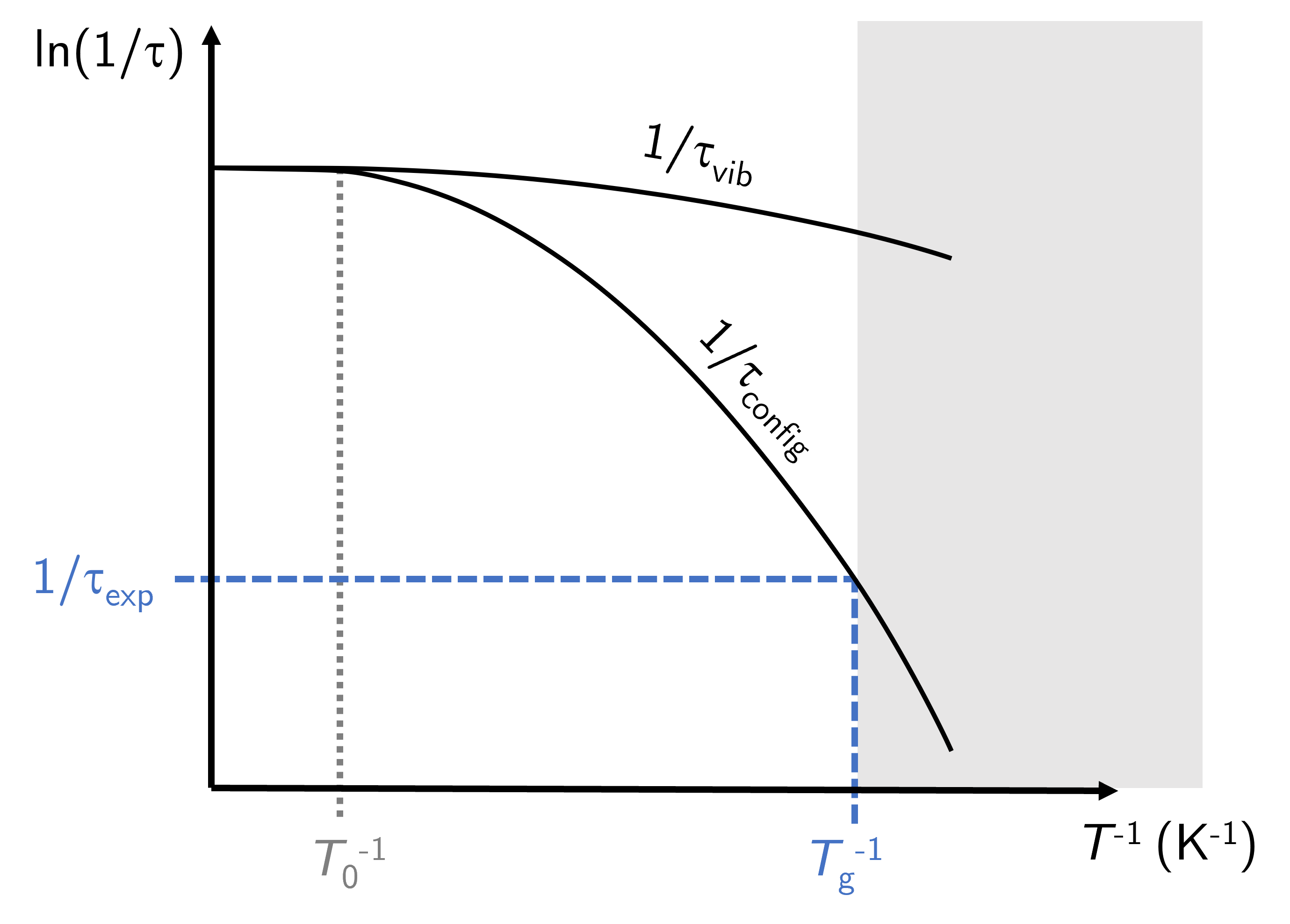
Fig. 12 Above a characteristic temperature \(T_0\) the vibrational and configurational timescales are similar. At lower temperatures these two timescales deviate, and subsequently the vibrational timescale is lower than that required for configurational changes.#
At temperatures above the Vogel-Fulcher temperature \(T_0\) the two lines overlap but as the system is cooled they begin to deviate. The configuration relaxation time increases much faster than the characteristic vibration time meaning the average time for conformational changes between molecules gets much longer with only a small decrease in temperature.
Now for the interesting effect. We live in a world in which our experimental observations take place above some finite timescale \(\tau_\text{exp}\): any process happening at timescales below this are not observed by us (even though they take place) and we only see the end result of the processes. As \(\tau_\text{config}\) increases so rapidly with decreasing temperature it follows that there will be some characteristic temperature in which the configurational relaxation is happening at timescales above \(\tau_\text{exp}\) and are, for all intents and purposes, not taking place fast enough for us to see the process happening. A good analogy here is the erosion of buildings due to rain - it is happening but at such a slow timescale that it appears to us that they are not eroding at all.
To stretch the analogy, we could see and measure the erosion if we had more sophisticated and precise experiments. What this does is change \(\tau_\text{exp}\) and if we can get this experimental timescale down to the same scale as erosion happens we will see it in action.
What this means then is that because the molecules in the liquid require longer timescales to rearrange than which we are observing the liquid for, the material behaves like a rigid material. The molecules are locked into their positions without any long range order but also without the time (strictly speaking the energy) to rearrange. The temperature that corresponds to this experimental timescale is the glass transition temperature \(T_g\). Or rather, it is one definition of \(T_g\). As I write these notes we still do not have a full understanding of the glass transition and there are differences between researchers as to what the glass transition is and what temperature we should be quoting for a given material.
Despite nobody in the world having a clear and definitive explanation of the glass transition process, we can still develop some insights and understanding from experimental data and how the proposed theories support or deviate from observations.
Measuring \(T_g\)#
There are two primary approaches used for determining the glass transition temperature of a material, measuring heat capacity and thermal expansivity. Both are used because they allow us to observe discontinuities in thermodynamic quantities that relate to the second derivatives of the free energy. We will consider each of these approaches separately both in terms of the underlying theory that drives the experimental process as well as some key findings from each technique.
\(T_g\) from thermal expansivity - Ellipsometry#
The key concept to remember here is that materials expand when they are heated and contract when cooled. Simple really.
If we have a liquid that is able to form a crystal then by cooling it down to a well-defined temperature, the melting temperature \(T_m\), the liquid then reduces in volume without any change in temperature. Once the atoms or molecules are all in a regular arrangement then the now solid will continue to shrink as it is cooled. This process is a first order phase transition and is characteristic for the solid-liquid transition. The thermal expansivity is the gradient of the temperature-volume curve and is linear for most materials (though different in the solid and liquid domains) - see Fig. 13.
Liquids that form glasses behave somewhat differently when cooled. In much the same way as a simple liquid behaves, a glass-forming liquid will contract when cooled, with a typically linear relationship that has a constant of proportionality of the expansion coefficient \(\alpha_\text{liquid}\). However when the temperature reaches the glass transition temperature there is a change in the gradient, and the new gradient is the expansion coefficient of the glass state \(\alpha_\text{glass}\). The key difference between crystal forming and glass forming liquids is that at the transition temperature the former has a decrease in volume that occurs at a constant temperature (the vertical segment of the black line in Fig. 13), corresponding to the latent heat required for the transition. The glass forming liquid only has a discontinuity in gradient without the vertical segment in the graph separating liquid and rigid phase.
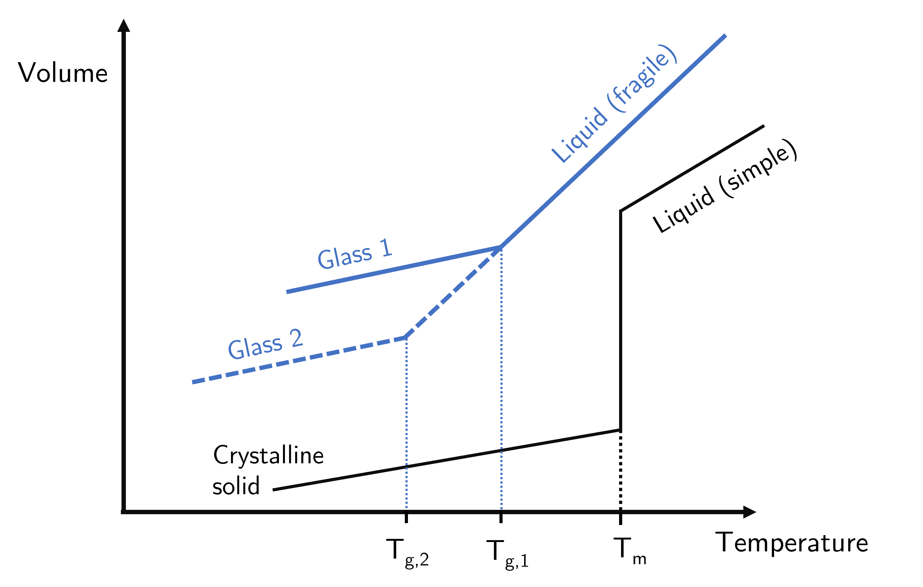
Fig. 13 Thermal expansion curves of a crystal-forming solid (black line) and a glass-forming material (blue lines). The melting temperature of the crystalline solid is a fixed value (for given pressure, etc) whereas the glass transition temperature varies depending on cooling rate, thermal history,…#
Some would say that the glass forming liquids have a second order phase transition because the transition is continuous rather than having a mixed-phased regime involving the latent heat. While this is true it is argued that the glass transition is not a true second order phase transition because it is not a fixed value for a given material.
A non-glass forming material that undergoes a second order phase transition (e.g. ferromagnetic transition, superconducting transition) will show the continuous transition but, and this is the important bit, it will always happen at the same temperature for any given material. So ferromagnetic material A will (generally) have a transition temperature at \(T_A\) regardless of the surrounding environment or factors. Glasses are much more fickle type of material in that their glass transition temperature depends strongly on factors such as the cooling rate, the number of times it has been heated and cooled, age of sample… So instead of trying to measure \(T_g\) for a given material, what glass transition scientists are trying to understand is how \(T_g\) is influenced by so many factors. To date we do not have a complete picture.
So now that we are armed with the foreknowledge that \(T_g\) is sensitive to experimental conditions, let us finally get to the substance of this section which is how to use ellipsometry to determine \(T_g\).
In short, ellipsometry uses the change in polarisation of light as it passes through a thin (\(\approx10-1000\text{ nm}\)) sample. The more material it passes through, the larger the change in polarisation between the p- and s- components, so we can reverse this experimentally to measure the change in polarisation to determine the amount (i.e. thickness) of the sample. This is quite neat but it gets even cooler when you then change the temperature of the sample. If you take thickness measurements across a range of temperatures you will get a set of data that looks like that in Fig. 13. We can then assume that \(T_g\) is at the point where the two lines (glass and liquid expansions with \(\alpha_\text{glass}\) and \(\alpha_\text{liquid}\) respectively) intersect.
This is a simplified model and we know that the transition process occurs over a finite temperature range roughly centred about \(T_g\) measured in this way, but this approach still gives some interesting insights. For example Keddie, Jones and Cory Keddie et al. [1994] found that the glass transition temperature of polystyrene depends on the thickness of a sample below about \(100\text{ nm}\). Their key result is shown in Fig. 14, and all each point on that graph is the glass transition temperature determined using the ellipsometry method we’ve just covered.
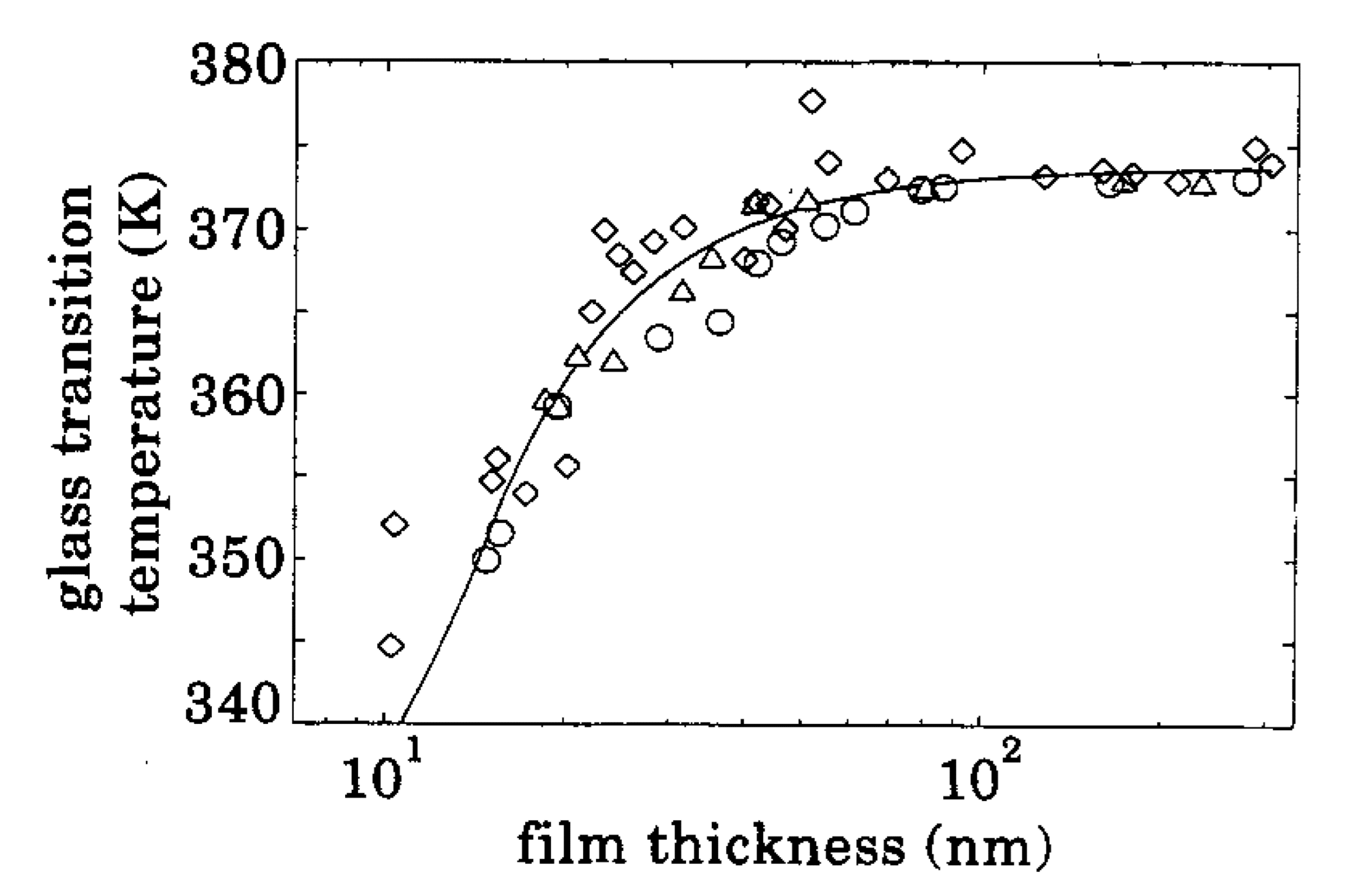
Fig. 14 First experimental evidence of the supression of \(T_g\) for ultrathin polymer films. \Taken from Keddie et al \cite{Keddie1994}#
It is worth re-emphasising the thickness range at which ellipsometry can be used. It is a great technique for testing thin film samples and surface effects but it is completely useless if we wanted to know more about the bulk properties of a material. For that we need another technique…
\(T_g\) from heat capacity - Differential Scanning Calorimetry#
…and here is another common technique in our \(T_g\) toolkit, one that works better for large, bulk materials rather than thin films.
Differential Scanning Calorimetry, or DSC, uses another fairly simple physical process but the devil is in the detail of developing suitably accurate equipment. The simple process that underpins this technique is that of heat capacity; adding a certain amount of heat to a sample will increase the temperature by some other amount, and the proportionality between heat and temperature change is the heat capacity.
The ‘calorimetry’ part of DSC is obvious here as we are talking about heat. But what about the ‘differential scanning’? The challenge experimentally is that new or unusual materials do not have a well established value for the heat capacity. To get around this issue the designers of DSC realised that you can extract information about your sample when you compare it to a well known reference sample.
In one method known as heat-flux DSC the sample and reference are placed in a temperature controlled chamber. The sample and reference are connected by a low–resistance heat–flow path. The assembly is enclosed in a single furnace. Enthalpy or heat capacity changesin the sample cause a difference in its temperature relative to the reference; the resulting heat
flow is small compared with that in differential thermal analysis (DTA) because the sample and reference are in good thermal contact. The temperature difference is recorded and related to enthalpy change in the sample using calibration experiments.
There are other types of DSC and refinements of the above, so if you are interested in the experimental and measurement side then I’d encourage you to look for some journal articles that used DSC.
When using DSC to determine \(T_g\) one would be interested in seeing how the specific heat capacity of the sample deviates away from a linear dependence with temperature. For example Schawe (Schawe [1995] and Fig. 15) used DSC to find the glass transition temperature for polystyrene, which you’ll also see agrees with those found in Fig. 14.
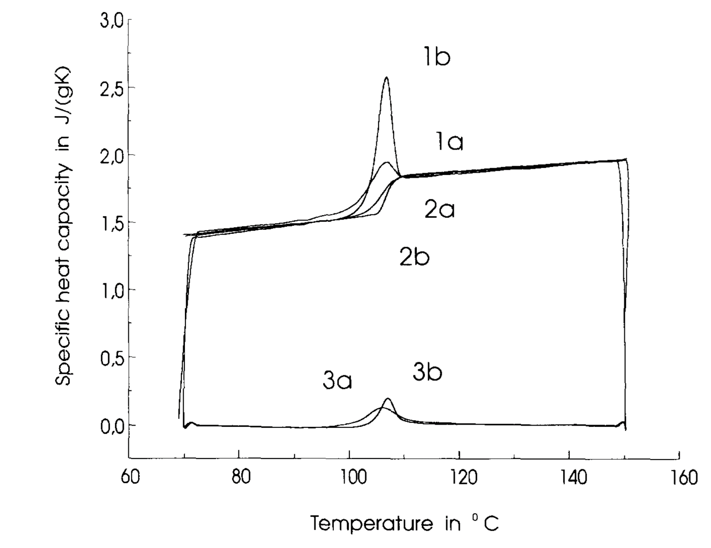
Fig. 15 The heat capacity of a material varies linearly below and above the transition temperature, but around \(T_g\) there is a noticible change that can either be a change in gradient (curves 2a and 2b) or even a peak in the curve (1a, 1b, 3a, 3b).#
Bibliography#
- KJC94
J. L. Keddie, R. A. L. Jones, and R. A. Cory. Size-Dependent Depression of the Glass Transition Temperature in Polymer Films. EPL (Europhysics Letters), 27(1):59, jul 1994. URL: https://iopscience.iop.org/article/10.1209/0295-5075/27/1/011 https://iopscience.iop.org/article/10.1209/0295-5075/27/1/011/meta, doi:10.1209/0295-5075/27/1/011.
- Sch95
J. E.K. Schawe. Principles for the interpretation of modulated temperature DSC measurements. Part 1. Glass transition. Thermochimica Acta, 261(C):183–194, sep 1995. doi:10.1016/0040-6031(95)02315-S.