2.3 Polymers: Real Chain

2.3 Polymers: Real Chain#

Excluded volume model#

So far we have considered the ideal chain case, and imposed some short-range restrictions between nearby monomers. However the ideal chain model does allow for a chain to loop back on itself such that segments that are widely separated along the chain could occupy the same region in space.
We shall now introduce another level of complexity to the model that prevents any segment from occuyping the same space - in essence we are ascribing a volume to each of our original bond vectors, and imposing the condition that volumes cannot overlap, and the presence of one volume excludes the possibility of another volume being found there.. This model is thus known as the excluded volume model model.

Let us return to the lattice model of a random walk system that we saw in Fig. 24, which I’m including here again to save you jumping between pages.

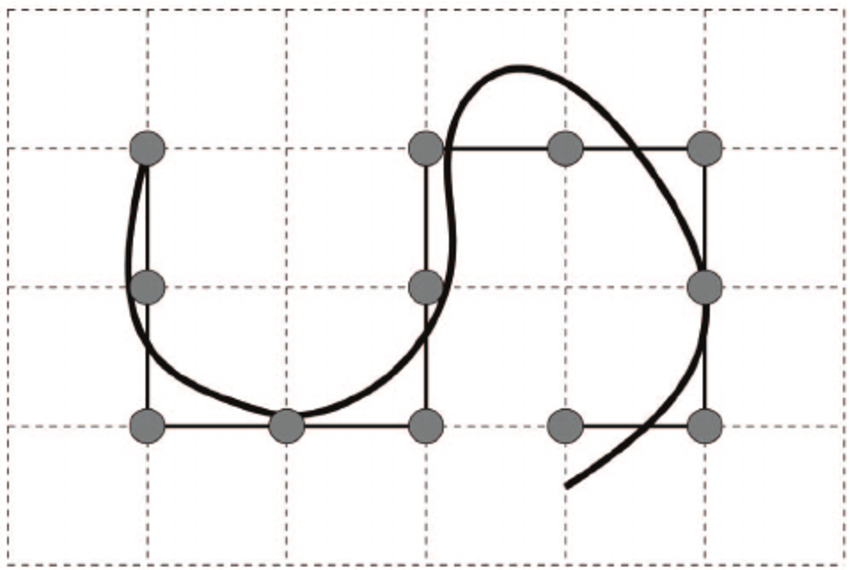
We can model a polymer chain (black) as a two-dimensional lattice where the ends of the segments are circles and as such the segments themselves lie only on the lattice lines.

Fig. 25 We can model a polymer chain (black) as a two-dimensional lattice where the ends of the segments are circles and as such the segments themselves lie only on the lattice lines.#

In the ideal case the end of the chain, which I am taking to be the point near the bottom right of the figure, could continue to the left and overlap the existing segments (the $4^\text{th}$ segment would be the first overlapped). Our short-range limitation would not prevent this new overlap because the overlapping segments are separated by a good number of other segments. Instead we need to move to a lattice model known as a self avoiding random walk that introduces the requirement that a segment cannot pass through any site that has been traversed previously. This imposition is realised by reducing the number of possible directions a segment step can take to the number of unoccupied adjacent sites.

Before we get into the detail, let us make a prediction to see how our intuition fares. The segments on an ideal chain can step in any of the directions available in the model used (in the 2D lattice, there are 4 directions available), whereas the real chain segments will have some directions removed from the possible options. As the chain grows in size we would expect the initial segments to be around the start of the chain, so the segments further along the chain will be required to occupy sites further from the start. In short, we would expect the volume occupied by a real chain to be larger than an ideal chain of the same length.

Excluded volume model#

In previous section we considered the ideal chain case, and imposed some short-range restrictions between nearby monomers. However the ideal chain model does allow for a chain to loop back on itself such that segments that are widely separated along the chain could occupy the same region in space.
We shall now introduce another level of complexity to the model that prevents any segment from occuyping the same space - in essence we are ascribing a volume to each of our original bond vectors, and imposing the condition that volumes cannot overlap, and the presence of one volume excludes the possibility of another volume being found there. This model is thus known as the excluded volume model model.

Let us return to the lattice model of a random walk system that we saw in Fig. 24 above but with some additions indicated in blue.

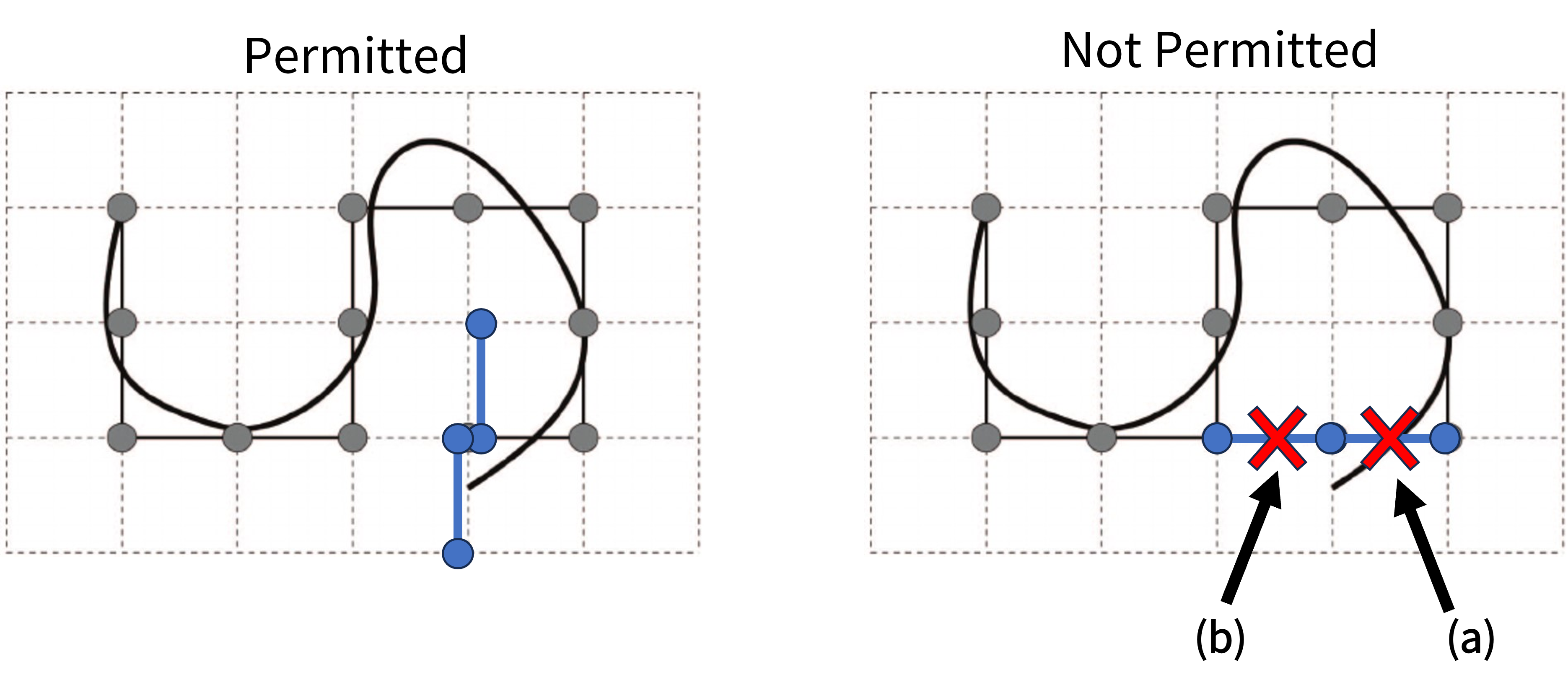
Fig. 26 There are two permitted places where an additional monomer can go, up or down from the end point. In the not permitted case option (a) (“doubling back”) is not permitted in either the short-range ideal or real case, whereas option (b) is permitted under the short-range ideal but not under the real chain model.#

In the ideal case a new momoner (blue) is added to the end of the chain, which I am taking to be the point near the bottom right of the figure could continue to the left and overlap the existing segments. The short-range limitation would not prevent this new overlap because the overlapping segments are separated by a good number of other segments. Instead we need to move to a lattice model known as a self avoiding random walk that introduces the requirement that a segment cannot pass through any site that has been traversed previously. This imposition is realised by reducing the number of possible directions a segment step can take to the number of unoccupied adjacent sites.

Before we get into the detail, let us make a prediction to see how our intuition fares. The segments on an ideal chain can step in any of the directions available in the model used (in the 2D lattice, there are 4 directions available), whereas the real chain segments will have some directions removed from the possible options. As the chain grows in size we would expect the initial segments to be around the start of the chain, so the segments further along the chain will be required to occupy sites further from the start. In short, we would expect the volume occupied by a real chain to be larger than an ideal chain of the same length.

Building the model in 3D#

Let us consider the total number of excluded volume chains whose $N^\text{th}$ step lies at a distance between $R$ and $R+\mathrm{d}R$ from the origin. I’ve shown this schematically in Fig. 27 where the blue chains meet this requirement but the yellow do not. We shall call this total number quantity $W(R)\,\mathrm{d}R$.

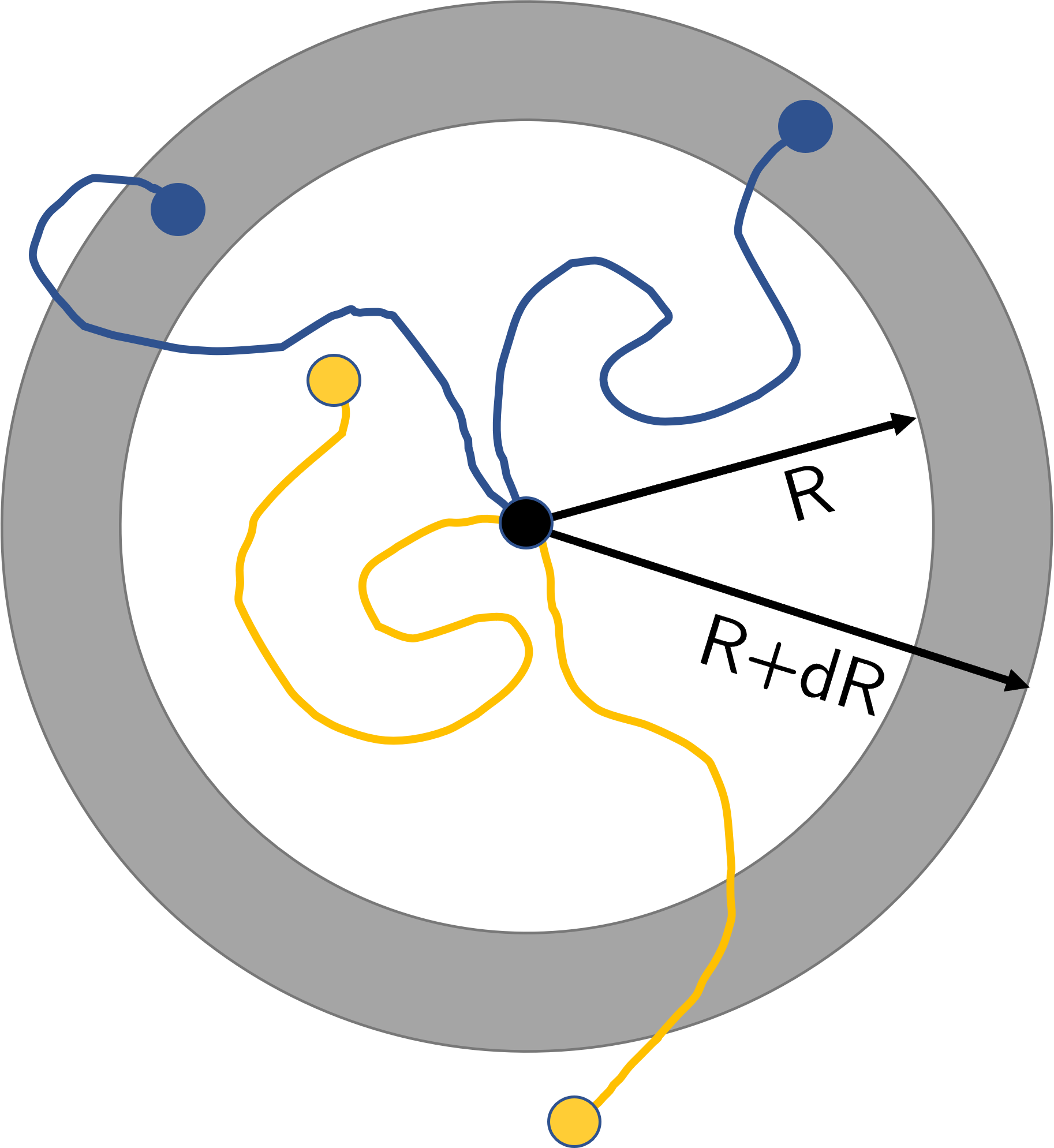
$We consider the number of chains whose $N^\text{th}$ step lies in the ring of inner radius $R$ and outer radius $R+\mathrm{d}R$ (the grey ring). The chains who meet this condition are in blue (the upper two chains) whereas those chains outside of this region of interest are in orange (lower two chains).$

Fig. 27 We consider the number of chains whose $N^\text{th}$ step lies in the ring of inner radius $R$ and outer radius $R+\mathrm{d}R$ (the grey ring). The chains who meet this condition are in blue (the upper two chains) whereas those chains outside of this region of interest are in orange (lower two chains).#

Since all possible paths have the same statistical weight, $W(R)$ is proportional to the distribution function of $R$ that we have already considered in previous sections.
In order to calculate $W(R)\,\mathrm{d}R$ we are going to take a conceptual step backwards and return to the ideal chain case. If we ignore the excluded volume effect then the total number of ideal chains with $N^\text{th}$ step lying at a distance between $R$ and $R+\mathrm{d}R$ is $W_0(R)\,\mathrm{d}R$. The total number of ideal chains with $N$ steps is $z^N$, and so the probability of the distance being between $R$ and $R+\mathrm{d}R$ is

\[P(\textbf{R},N)\,4\pi R^2\,\mathrm{d}R\]

where $P(\textbf{R},N)$ has previously been defined (equation (20)). Therefore we find

(22)#\[W_0(R) = z^N4\pi R^2 \left(\frac{3}{2\pi Na^2}\right)^{\frac{3}{2}}\,\exp\left(-\frac{3R^2}{2Na^2}\right)\]

Our next step is to recognise that there will be some subset of these ideal configurations that are not allowed under the excluded volume condition. Let us use $p(R)$ as the probability that an ideal chain configuration (as counted in equation (22)) is also allowable under the excluded volume condition.

We estimate $p(R)$ by assuming that the polymer segments are evenly distributed in a region of volume $R^3$, which means there are $\dfrac{R^3}{v_c}$ lattice sites where $v_c$ is the volume of a single lattice element. We can now calculate the probability that no overlaps occur if we place $N$ segments on these lattice sites.
The probability that one particular segment will not overlap with another is $\left(1-\frac{v_c}{R^3}\right)$ and since there are $\dfrac{N(N-1)}{2}$ possible combinations of segment pairs the probability that no overlap occurs in all of these combinations is

(23)#\[\begin{split}p(R) &= \left(1-\frac{v_c}{R^3}\right)^{\frac{N(N-1)}{2}}\nonumber\\ &= \exp\left( \ln\left[\left(1-\frac{v_c}{R^3}\right)^{\frac{N(N-1)}{2}}\right] \right)\nonumber\\ &= \exp\left(\frac{N(N-1)}{2}\,\ln\left(1-\frac{v_c}{R^3}\right)\right)\end{split}\]

Here we can make two simplifications. The first is that when $R^3\gg v_c$ then $\ln\left(\dfrac{v_c}{R^3}\right)\approx \dfrac{v_c}{R^3}$, and secondly if $N\gg 1$ then $N(N-1)\approx N^2$. Using both of these approximations simplifies equation (23) as

(24)#\[p(R) = \exp\left(-\frac{N^2v_c}{2R^3}\right)\]

Let us take a moment to recentre ourselves in what we are trying to establish. Equation (24) tells us the probability that a configuration in the ideal chain conditions is also allowed under the excluded volume condition. So the product of this probability and the number of ideal chain configurations $W_0(R)$ (equation (22)) will be the number of configurations allowed in the excluded volume conditions, i.e.

(25)#\[\begin{split}W(R) &= W_0(R)\,p(R)\\ &\propto R^2\,\exp\left(-\frac{3R^2}{2Na^2}-\frac{N^2v_c}{2R^3}\right)\end{split}\]

where for equation (25) I’ve dropped a number of prefactors and constants to simplify it to the proportionality that is of interest.

Both $W(R)$ and $W_0(R)$ have a maximum for a certain value of $R$ which will tell us the most likely size of the real and ideal chains respectively. We can find these maxima, which I will label $R^*$ and $R_0^*$ respectively, using a bit of calculus.

Finding $R_0^*$ is fairly trivial, in that we use part of equation (22) with

\[\begin{split}0 &= \frac{\mathrm{d}W_0(R)}{\mathrm{d}R}\bigg\rvert_{R=R_0^*}\\ &= \frac{\mathrm{d}}{\mathrm{d}R}\left[R^2\,\exp\left(-\frac{3R^2}{2Na^2}\right)\right]\bigg\rvert_{R=R_0^*}\\ &= 2R_0^*\left(1-\frac{3(R_0^*)^2}{2Na^2}\right)\exp\left(-\frac{3(R_0^*)^2}{2Na^2}\right)\end{split}\]

for which there are three conditions in which the equality can hold: $R_0^*=0$, $R_0^*\rightarrow\infty$ and

(26)#\[\begin{split}0 &= \left(1-\frac{3(R_0^*)^2}{2Na^2}\right)\\ \therefore R_0^* &= \sqrt{\frac{2Na^2}{3}}\\ &= \sqrt{\frac{2}{3}}aN^{\frac{1}{2}}\end{split}\]

The reason I’ve rearranged into the final step is simply to highlight how this relationship is almost identical to the one we found for the ideal chain case (equation (17)). It is somewhat reassuring that the two different approaches, namely a vector average and a probability distribution approach, give the same form of relationship with only a numerical prefactor difference.

Moving on now to the excluded volume case. Once again we can find $R^*$ via calculus but this time we start from equation (25). This is a bit more complicated to differentiate directly, although you can do it if you want the practice, but I instead will instead look for the maximum in the natural logarithm of equation (25).

\[\begin{split}\ln W(R) = \ln\left[ R^2\,\exp\left(-\frac{3R^2}{2Na^2}-\frac{N^2v_c}{2R^3}\right) \right] &= -\frac{3R^2}{2Na^2}-\frac{N^2v_c}{2R^3} +2\ln R\\ \therefore \frac{\mathrm{d}\left(\ln W(R)\right)}{\mathrm{d}R}\bigg\rvert_{R=R^*} &= -\frac{3R^*}{Na^2}+\frac{3N^2v_c}{2(R^*)^4}+\frac{2}{R^*}=0\\\end{split}\]

Rearranging this expression gives

(27)#\[-\frac{3(R^*)^2}{2Na^2}+\frac{3N^2v_c}{4(R^*)^3}+1=0\]

Throughout the construction of this model we have been comparing the ideal chain case with the excluded volume case. Thus we combine equations (27) and (26) to find an expression for the ratio of the two sizes,

\[\left(\frac{R^*}{R_0^*}\right)^5-\left(\frac{R^*}{R_0^*}\right)^3=\frac{\sqrt{486}}{16}\frac{v_c}{a^3}\sqrt{N}\]

In the case that $N\gg 1$ then the first term on the left hand side is much larger than the second term, so we can drop the cubic bracket and simplify the remaining expression as

(28)#\[\begin{split}R^* &\approx R_0^*\left(\frac{N^{\frac{1}{2}}v_c}{a^3}\right)^{\frac{1}{5}}\\ &\propto N^{\frac{3}{5}}\end{split}\]

There we have it. Our excluded volume model of a real chain predicts that the size of the polymer is proportional to $N^{\frac{3}{5}}$ rather than the $N^\frac{1}{2}$ predicted by the ideal chain model.

In general then our simple models are predicting a relationship that has the following form:

\[R \approx N^\nu b\]

and what is most surprising is that years of experimental data and sophisticated numerical simulations put the exponent value to be approximately $0.588$, which is pretty darn close to the $\frac{3}{5}=0.6$ we found from a fairly simple excluded volume model.

(Re)building the real chain model.#

I’m going to rederive an expression for the real chain but using a different approach, namely one where the energy of the system is considered. The reason why I am doing it again, and why I’m presenting this approach second, is that it is one of those models that requires a good grasp of important but nebulous ideas. These ideas will be better reinforced throughout the module so you may find that this derivation is less obvious first time through but is clearer and more simple when you come to re-read it at the end of the course.

We start again from the idea that our $N$ segments are uniformly distributed across some volume $R^3$. Thus the concentration of segments $c$ is approximately

\[c\sim\frac{N}{R^3}\]

I say approximately because there may be some prefactors that give an exact answer when taking into account the rough “surface” of the volume and restrictions on packing segments into the volume. But we can confidently state that the concentration varies with $N$ and inversely with $R^3$.
The effective repulsion between segments, $F_\text{rep}$, makes a positive contribution to the free energy, and this contribution is proportional to both the concentration and the number of segments. So

\[\begin{split}F_\text{rep} &\propto cN\\ &\propto \frac{N}{R^3}N\\ &= k_\text{B}Tb\frac{N^2}{2R^3}\end{split}\]

where $b$ is a constant of proportionality and has dimensions of volume. The $k_\textbf{B}T$ has been included for two reasons: to give the expression the correct units, but more importantly the excluded volume effect is (broadly speaking) entropic in origin.

So if the repulsions between segments makes this positive contribution to the free energy of the chain, why does the whole chain not expand until it is a single straight line? This configuration would give the smallest possible interaction between segments and consequently minimise the free energy. The answer is entropy - by limiting the possible states a segment can be in we would decrease the associated entropy. Having a larger entropy will also reduce the free energy of the system, so our chain will try to find a happy medium state between minimising the repulsive interaction between segments and increasing the entropy of the chain.
We can model the entropy, $S$, as an entropic spring (from equation (20)) which in turn gives an associated contribution to the free energy

(29)#\[\begin{split}S &= -\frac{3k_\text{B}r^2}{2Na^2} + \text{constant}\\ \therefore F_\text{el} &= k_\text{B}T\frac{r^2}{Na^2}\end{split}\]

I’ve given the vague statement that the polymer will find this “happy medium” between repulsion and elastic entropy, but we can formalise this mathematically. The optimal configuration of the polymer is the one that minimises the total free energy $F_\text{total} = F_\text{rep}+F_\text{el}$. Thus

\[\begin{split}F_\text{total} &= k_\text{B}Tb\frac{N^2}{2R^3} + k_\text{B}T\frac{R^2}{Na^2}\\ &= k_\text{B}T\left(\frac{bN^2}{2R^3} + \frac{R^2}{Na^2}\right)\\ \therefore \frac{\mathrm{d}F_\text{total}}{\mathrm{d}R} &= k_\text{B}T\left(\frac{2R}{Na^2}-\frac{3bN^2}{2R^4}\right) = 0\end{split}\]

Assuming that $k_\text{B}T\neq0$, the term within the bracket must equal zero and so

\[\begin{split}\frac{2R}{Na^2}&=\frac{3bN^2}{2R^4}\\ R^5 &= \frac{3a^2b}{4}N^3\\ \therefore R &= \left(\frac{3a^2b}{4}\right)^{\frac{1}{5}}N^{\frac{3}{5}}\\ \text{or } R &\propto N^\frac{3}{5}\end{split}\]

Exactly the same result as found previously (equation (28))!

Homework hint

For one of the homework questions you are asked to comment on why we expect a different value for $\nu$ depending on the dimensionality of the self avoiding random walk (i.e. 2D versus 3D), and why this doesn’t happen for the ideal case.

To answer this have a look through the two different ways of deriving the 3D self avoiding random walk result (i.e. probability method and energy method) and find terms that relate to volume and surface area of 3D shapes.

Note that the question doesn’t require you to fully derive the result for the 2D case, but this is one approach you could take if you prefer the quantitative method over the qualitative description.

Effect of solvent and the $\Theta$ temperature#

Interactions with solvent.#

It will probably come as no surprise to you that most polymers in the world do not exist in a vacuum. I know, right!? But in all of the models we have seen so far we have only considered whether the units or segments of a polymer chain occupy a space on the lattice or not. What we need to consider next is that when a polymer is found surrounded by some other material, and for the purposes of this course we will only consider polymers surrounded by solvent or by other polymers.
We will focus on the polymer in solvent case. Returning to the lattice model this means that lattice sites are occupied either by a polymer segment or a solvent molecule. In Fig. 28 the real polymer chain is depicted in black and white circles are solvent molecules. For simplicity we will assume that the polymer segments (p) and solvent molecules (s) have the same volume and can only occupy a single site on the lattice, and that there are no empty sites.

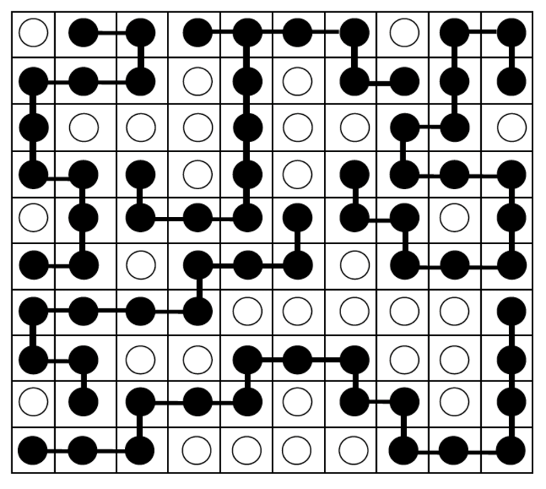
We can expand the two-dimensional lattice model to include solvent molecules. The polymer chain lies on the lattice lines, with their ends indicated with black circles and aligned with the centre of a lattice unit. Any unit not occupied with a polymer end is filled with a solvent molecule (white).

Fig. 28 We can expand the two-dimensional lattice model to include solvent molecules. The polymer chain lies on the lattice lines, with their ends indicated with black circles and aligned with the centre of a lattice unit. Any unit not occupied with a polymer end is filled with a solvent molecule (white).#

The interaction energies between neighbouring elements on the lattice are:

$-\epsilon_{pp}$ = polymer-polymer interactions
$-\epsilon_{ps}$ = polymer-solvent interactions
$-\epsilon_{ss}$ = solvent-solvent interactions

These energies originate from the van der Waals interaction and so are all positive.
For a given configuration of the chain $i$, let $N_{pp}^i$ be the number of neighbouring polymer-polymer pairs on the lattice. Similarly $N_{ps}^i$ and $N_{ss}^i$ are the number of neighbouring polymer-solvent and solvent-solvent parts respectively. Thus the total energy of the system for this configuration $E_i$ is given by

(30)#\[E_i = -N_{pp}^i\epsilon_{pp} -N_{ps}^i\epsilon_{ps} -N_{ss}^i\epsilon_{ss}\]

Now that we are considering the additional interactions between polymer-solvent and solvent-solvent, the probability of a real chain having size $R$ is no longer proportional to $W(R)$ but instead needs to be modified by a thermodynamic term, namely

(31)#\[P(R) \propto W(R)\,\exp\left(-\frac{\left<E(R)\right>}{k_\text{B}T}\right)\]

where $\left<E(R)\right>$ is the average energy of a polymer of size $R$.

We again assume that the polymer segments are uniformly distributed in a region of volume $R^3$ so that the probability of a lattice site being occupied by a polymer segment $\phi$ is

\[\phi=\frac{Nv_c}{R^3}\]

Therefore the average number of pairs can be estimated as:

\[\begin{split}\left<N_{pp}^i\right> &\approx \frac{1}{2}zN\phi\\ \left<N_{ps}^i\right> &\approx zN(1-\phi)\\ \left<N_{ss}^i\right> &\approx N_{ss}^0 - \left(\left<N_{pp}^i\right> + \left<N_{ps}^i\right>\right)\\ &= N_{ss}^0-\left[\frac{1}{2}zN\phi + zN(1-\phi)\right]\end{split}\]

where $N_{ss}^0$ is the numer of pairs of neighbouring solvent molecules when there is no polymer molecule in the system.
Substituting these three expressions into equation (30) gives us the following expression for the average energy of a polymer of size $R$

(32)#\[\begin{split}\left<E(R)\right> &\approx -\frac{1}{2}zN\phi\left(\epsilon_{pp}+\epsilon_{ss}-2\epsilon_{ps}\right) + \text{terms independent of }\phi\\ &= -\frac{zN^2v_c}{R^3}\Delta \epsilon + \text{terms independent of }\phi\end{split}\]

where $\Delta \epsilon$ is defined as

(33)#\[\Delta \epsilon = \frac{1}{2}\left(\epsilon_{pp}+\epsilon_{ss}\right)-\epsilon_{ps}\]

We can substitute our expression for the energy is the polymer (equation (30)) and the number of states $W(R)$ (equation (25)) into our expression for the probability of a chain having a size $R$ (equation (31)) to find

(34)#\[\begin{split}P(R) &\propto R^2\,\exp\left(-\frac{3R^2}{2Na^2}-\frac{N^2v_c}{2R^3}\right)\,\exp\left(\frac{zN^2v_c\Delta\epsilon}{k_\text{B}TR^3}\right)\\ &= R^2 \exp\left(-\frac{3R^2}{2Na^2}-\frac{N^2v_c}{2R^3}+\frac{zN^2v_c\Delta\epsilon}{k_\text{B}TR^3}\right)\\ &= R^2 \exp\left(-\frac{3R^2}{2Na^2} - \frac{N^2v_c}{2R^3}\left(1 - \frac{2z\Delta\epsilon}{k_\text{B}T}\right)\right)\\ &= R^2 \exp\left(-\frac{3R^2}{2Na^2} - \frac{N^2v_c}{2R^3}\left(1 - 2\chi\right)\right)\end{split}\]

where $\chi=\dfrac{z\Delta\epsilon}{k_\text{B}T}$ is a dimensionless quantity known as the interaction parameter. We will explore what this parameter really means more when we come to study phase transitions and liquid-liquid unmixing.

Finally let us compare equation (31) here with that found in the excluded volume model (equation (25)). By comparing these two equations we can combine the effects of excluded volume and solvent interactions into a single parameter known as the excluded volume parameter $v$

(35)#\[\begin{split}v &= v_c\left(1-2\chi\right)\\ &= v_c\left(1-\frac{2z}{k_\text{B}T}\Delta\epsilon\right)\end{split}\]

$\Theta$ temperature.#

Take a few moments to think about what equation (35) actually tells us. The parameter $v$ not only depends on excluded volume effects (through $v_c$ and partly through $z$) but also on the effections of solvent interactions as expressed by $\Delta \epsilon$.

Let us see how $\Delta \epsilon$ relates to changes in our lattice configuration. In Fig. 29 we have two polymer segments (black circles) in amongst solvent molecules (white circles) - for simplicity we are only considering single polymer units rather than the full chain.

Initially the two polymer segments (black) are separated such that there are solvent molecules between them (left-hand side of image). Each polymer is interacting with four nearest neighbour solvent molecules. We then move the polymer segments to adjacent lattice spaces meaning the polymer segments now only interact with three solvent molecules but also with one polymer segment (right-hand side of image)

Fig. 29 Initially the two polymer segments (black) are separated such that there are solvent molecules between them (left-hand side of image). Each polymer is interacting with four nearest neighbour solvent molecules. We then move the polymer segments to adjacent lattice spaces meaning the polymer segments now only interact with three solvent molecules but also with one polymer segment (right-hand side of image)#

In part (a) of the figure we have two polymer segments that are initially separated, meaning they are completely surrounded by solvent molecules. We assume that molecules can only interact with their nearest neighbours, just to keep things simple. Then we move the right hand polymer molecule to the left, switching places with the solvent molecule that was originally there. This has three effects on the energy of the system:

add a polymer-polymer interaction, $+\epsilon_{pp}$
item add a solvent-solvent interaction, $+\epsilon_{ss}$
item remove two polymer solvent interactions, $-2\epsilon_{ps}$

The third of these comes from the polymers originally interacting with 4 solvent molecules each but then having one of these interactions each replaced with a polymer-polymer interaction. Thus the total change in energy is

\[\epsilon_{pp}+\epsilon_{ss} - 2\epsilon_{ps} = 2\Delta\epsilon\]

where we have pulled in the definition from equation (33) here.

This tells us that if $\Delta\epsilon >0$ then the polymer segments will tend to aggregate together - the polymer-polymer interaction energy is greater than polymer-solvent interactions. In the case where $\Delta\epsilon<0$ then the interactions between polymer-solvent molecules is greater meaning the polymer will tend to “dissolve” into the solvent.

In a good solvent $\Delta\epsilon$ is small such that $v$ is always positive - this is implied within the definition of what a good solvent is. A good solvent by definition has a favourable interaction with the polymer, which is why the polymer will “dissolve” in it.

In a poor solvent we find that $\Delta\epsilon$ is large as the energy of polymer-polymer and solvent-solvent interactions are much larger than polymer-solvent ones. This leads to an interesting result when we consider equation (35) again. When $\Delta\epsilon$ is sufficiently large (of order $10^{-21}\text{ J}$) then under typical experimental conditions we are in the realm of $\Delta\epsilon\sim k_\text{B}T$. Consequently there exists some temperature for a system with some $\Delta\epsilon$ and $z$ such that the bracket term in equation (35) becomes zero. This temperature, known as the $\Theta$ temperature, is the temperature1 at which the excluded volume parameter $v$ equals zero, meaning the repulsive excluded volume effect perfectly balances the attractive force between the segments. At the theta temperature the polymer behaves as an ideal chain. Finally we can define an expression for $\Theta$ using equation (35) under the condition that $v=0$

\[\Theta = \frac{2z\Delta\epsilon}{k_\text{B}}\]

You’ll be reassured to know that this checks out in experimental data. One of the earliest studies [Sun et al., 1980] looked how the radius of polystyrene molecules changes with temperature.

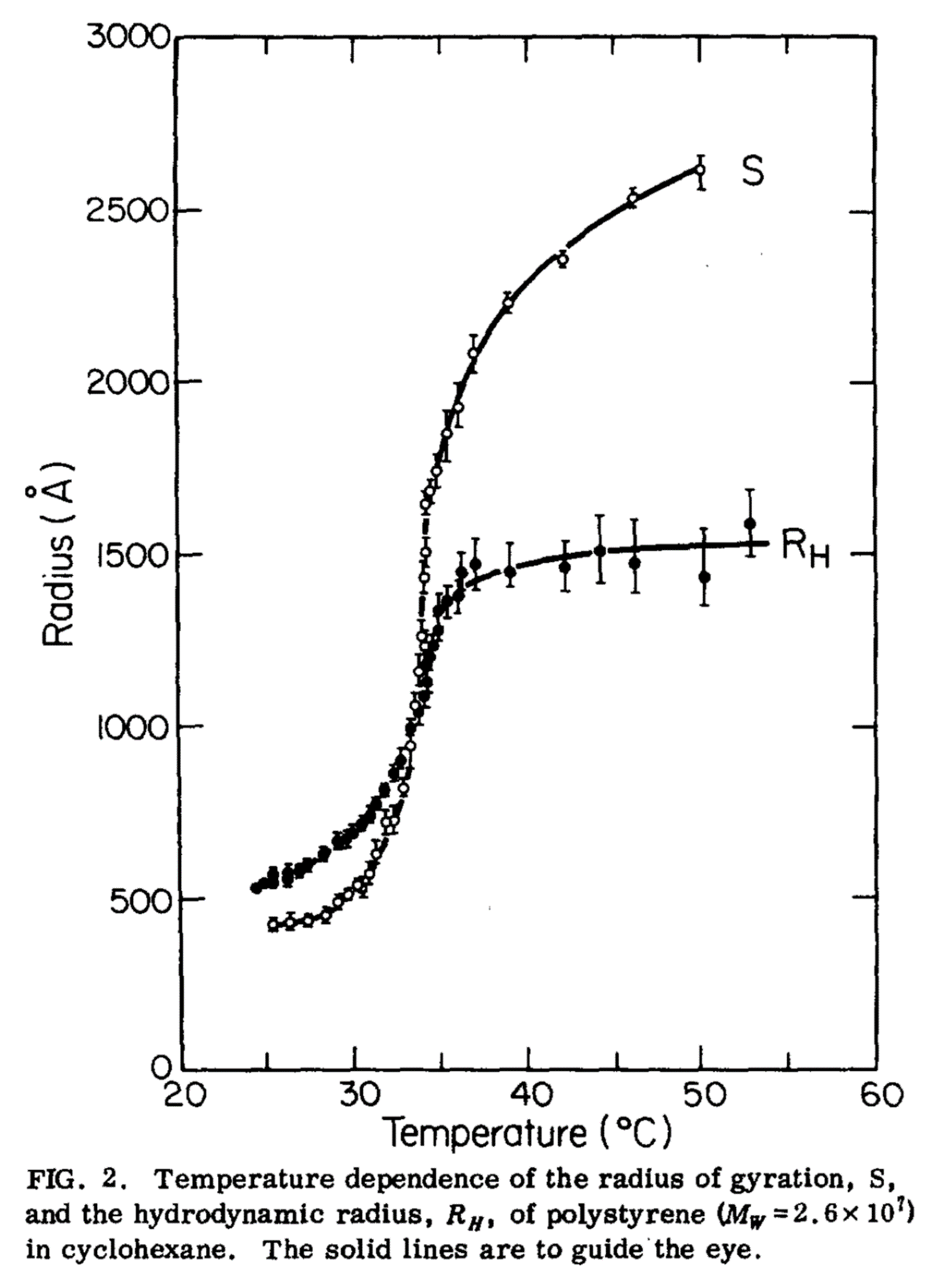
The radius of gyration and hydrodynamic radius of polystyrene measured as a function of temperatue. At the theta temperature there is a sharp increase in both types of radius.

Fig. 30 The radius of gyration and hydrodynamic radius of polystyrene measured as a function of temperatue. At the theta temperature there is a sharp increase in both types of radius. Taken from [Sun et al., 1980], and includes their original caption.#

The data are shown in Fig. 30 and show a marked change in the radius of the polymer around the theta temperature of $35^\circ\text{C}$ compared to the smaller changes at temperatures above and below $\Theta$. There is still a temperature dependence on the radius, but the gradient $\dfrac{\mathrm{d}R}{\mathrm{d}T}$ is largest at $T=\Theta$.

Beyond single polymers - dilute vs concentrated.#

In all of the previous sections we have considered the individual polymer chain, how it moves and how it responds to changes in environment. But what happens when we have a few chains? What about a few more? And what about a lot?

To try and impose some structure to our discussions we will define the different concentration domains of a polymer in solvent solution, as shown in Fig. 31. At one extreme end we have no polymer chains whatsoever meaning the system is pure solvent. Next we have a dilute system in which the small number of polymer chains in the solutions are, on average, sufficiently separated that they do not interact with each other. We next have the semi-dilute where chains begin to overlap and interact, but there are still distinct regions of pure solvent. Next we have the concentrated solution in which the polymer chains and solvent are uniformly distributed in the solution. Finally we have the other extreme of a pure polymer system in which there is no solvent whatsoever.

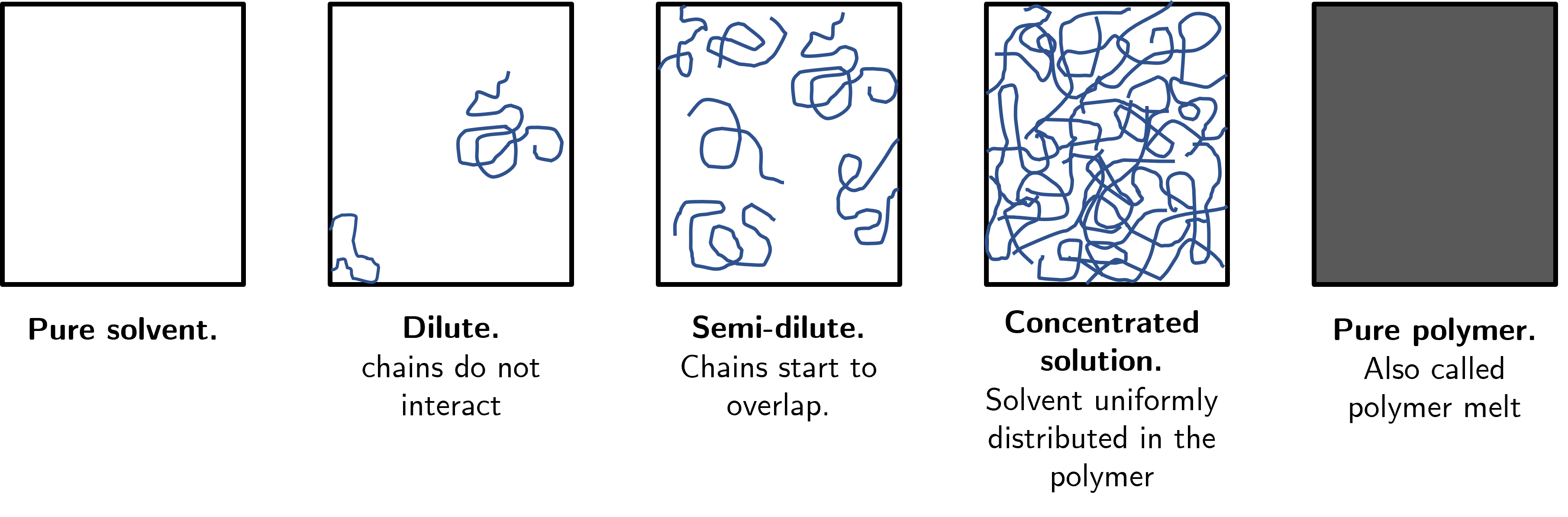
Fig. 31 Five broad domains of polymer solutions, ranging from pure solvent (left) to pure polymer (right).#

In the dilute regime the polymers do not follow random walk statistics as excluded volume effects cause the chain to swell. Somewhat counterintuitively, the system becomes easier to model as the solution becomes more and more concentrated; in the polymer melt and concentrated systems the chains follow ideal random walk statistics.

We’ll take an argument from Flory who considered the segment concentration $c$ across a one-dimensional ‘slice’ of our solution, which we will align along $x$. The excluded volume effect introduces an unfavourable energy of interaction that is proportional to the probability of two segments being close together, i.e. proportional to $c^2$. This leads to a force on the segments proportional to $c\,\frac{\mathrm{d}c}{\mathrm{d}x}$.

Now take a look at Fig. 32. This force is proportional to the gradient of the concentration-position curves. In the dilute regime the gradient is large but as segments start to overlap the gradient decreases. Once in the concentrated domain there are no large gradients in the concentration2 which thus tells us the excluded volume effect is no longer involved.

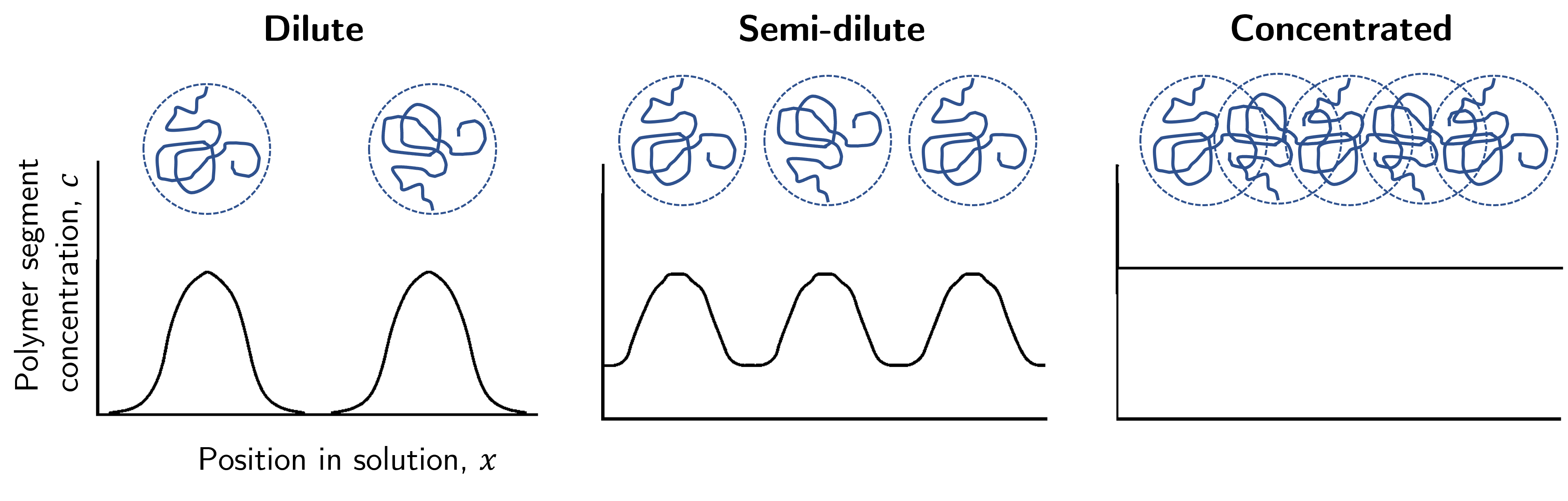
In the dilute domain the segment concentration has a large concentration gradient between polymer and solvent. As the solution becomes more concentrated these gradients decrease, and in the concentrated domain there is no concentration gradient throughout the solution.

Fig. 32 In the dilute domain the segment concentration has a large concentration gradient between polymer and solvent. As the solution becomes more concentrated these gradients decrease, and in the concentrated domain there is no concentration gradient throughout the solution.#

Summary - Polymer types, sizes and solutions#

So that concludes our work in understanding how big a polymer chain is, and how we differentiate between dilute polymer systems and concentrated / polymer melt systems. Seems like a lot of effort and maths, but what I hope you can take away from this is that we are able to develop some models based on fairly simple premises that lead to a surprisingly good estimate when compared to results from simulations and experiments.

1: Yes, three “temperatures” in a row. I couldn’t figure a better way to phrase it…
2: For the sake of completeness, there may be local fluctuations in concentration due to thermodynamics. This can lead to interesting effects but for the purpose of this thought experiment we can neglect them.

2.3 Polymers: Real Chain

Contents

2.3 Polymers: Real Chain#

Excluded volume model#

Excluded volume model#

Building the model in 3D#

(Re)building the real chain model.#

Effect of solvent and the \(\Theta\) temperature#

Interactions with solvent.#

\(\Theta\) temperature.#

Beyond single polymers - dilute vs concentrated.#

Summary - Polymer types, sizes and solutions#

Bibliography

- SNST80(1,2)
Shao‐Tang Sun, Izumi Nishio, Gerald Swislow, and Toyoichi Tanaka. The coil–globule transition: radius of gyration of polystyrene in cyclohexane. The Journal of Chemical Physics, 73(12):5971–5975, 1980. URL: https://doi.org/10.1063/1.440156, arXiv:https://doi.org/10.1063/1.440156, doi:10.1063/1.440156.